Visual Understanding of Insertion Sort Algorithm
Category > Algorithms
Sep 01, 2020In computer science, a sorting algorithm is an algorithm that puts elements of a list in a certain order. Efficient sorting is important for optimizing the efficiency of other algorithms (such as search and merge algorithms) that require input data to be in sorted lists. Sorting is also often useful for canonicalizing data and for producing human-readable output. - From Wikipedia
There are many sorting algorithms. One of the most important factor when choosing which sorting algorithm to use is its algorithm complexity, represented in Big-O notations. Figure (1) summarizes the the algorithm complexity of various sorting methods. Note that $N$ is is an array size, $O$ is the worst-case scenario, $\Omega$ is the best-case scenario, and $\theta$ is the average-case scenario. This post focuses on Insertion Sort.
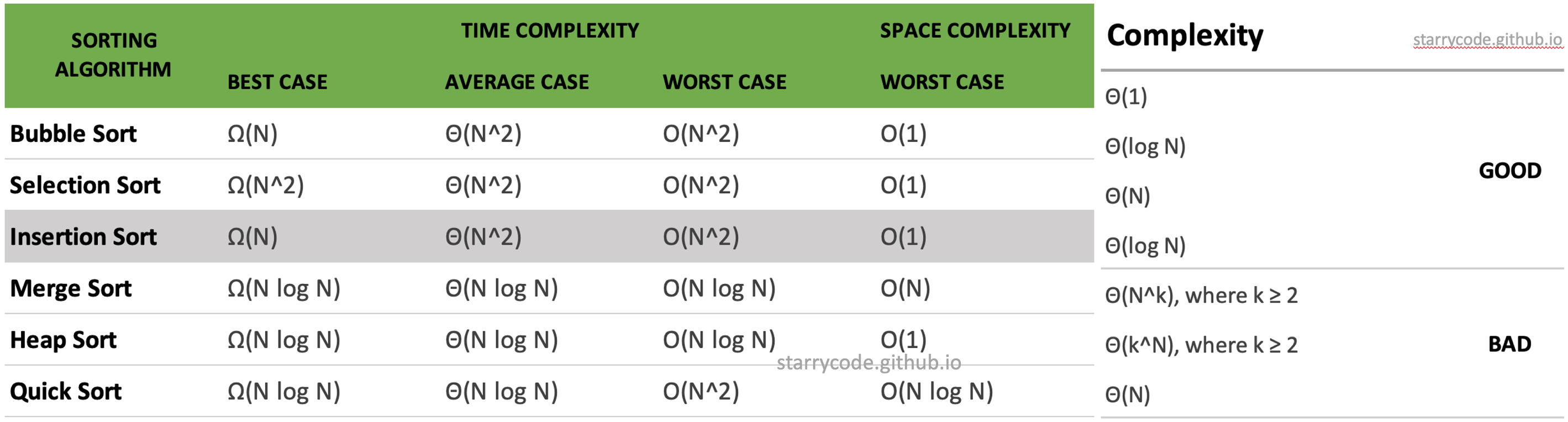
Figure 1: Algorithm complexities and their efficiencies
1. Insertion Sort
Insertion sort is an in-place comparison-based algorithm. In the best case scenario, in which the array is nearly-sorted, it has $O(N)$ time complexity. In the worst case scenario, in which the array is reserve-sorted, it has $O(N^2)$ time complexity, according to figure (1). It has the following pros and cons:
Pros
- When array size is small, insertion sort is faster than divide-and-conquer algorithms (quicksort, mergesort, heapsort), because they have extra overhead from the recursive function calls.
- If data is almost sorted, it can be very fast, approaching $O(N)$ time complexity
- In-place; i.e., only requires a constant amount of $O(1)$ of additional memory space
- More efficient in practice than most other simple quadratic $O(N^2)$ algorithms such as selection or bubble sort.
- Simple and easy to implement
Cons
- Bad for large data sets due to its quadratic nature $O(N^2)$.
- Writes more than selection sort $O(1)$, whereas insertion is $O(N^2)$.
1.1. Understanding Insertion Sort
Insertion sort works in a similar way that you sort playing cards in your hands. The algorithm searchs an array sequentially, and elements in the unsorted sub-list is inserted into the sorted sub-list. Similar to selection sort, the algorithm divides the list into two parts:
The sub-list which is already sorted.
Remaining sub-list which is unsorted.
An element which is to be 'inserted' in this sorted sub-list, has to find its appropriate position to be inserted, by comparing itself to its predecessor. Hence the name, insertion sort. Note that insertion sort is very similar to selection sort.
Let's dive into the illustrations for better understanding of insertion sort. Imagine that you want to sort the books shown in figure (2) in ascending order of sizes.
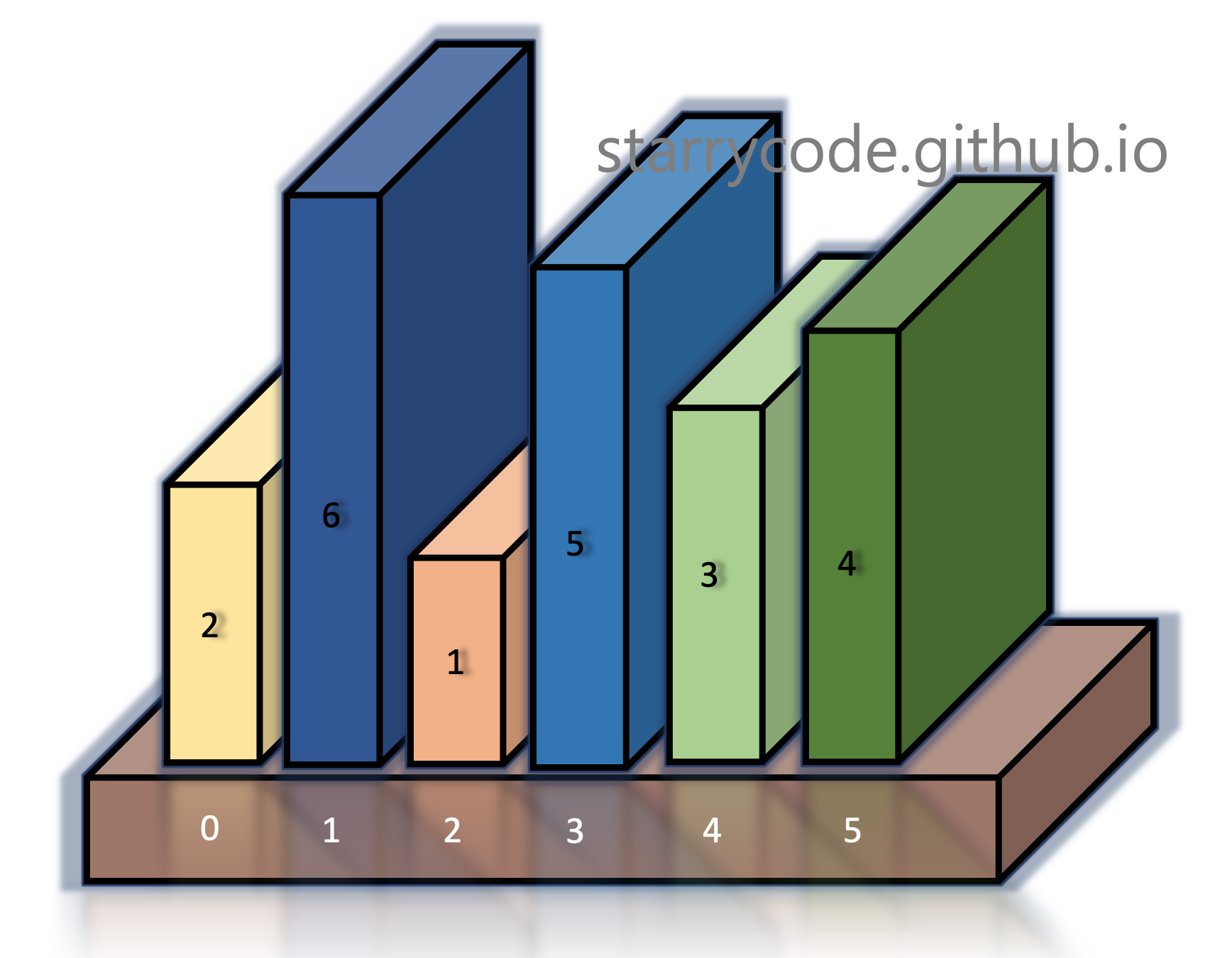
Figure 2: Books to sort
1st Iteration
Insertion sort divides a list into sorted & unsorted sublists. The grey divider represents the split between sorted (left) vs unsorted (right) array. At the beginning, nothing is sorted. We move the divider one index to the right.
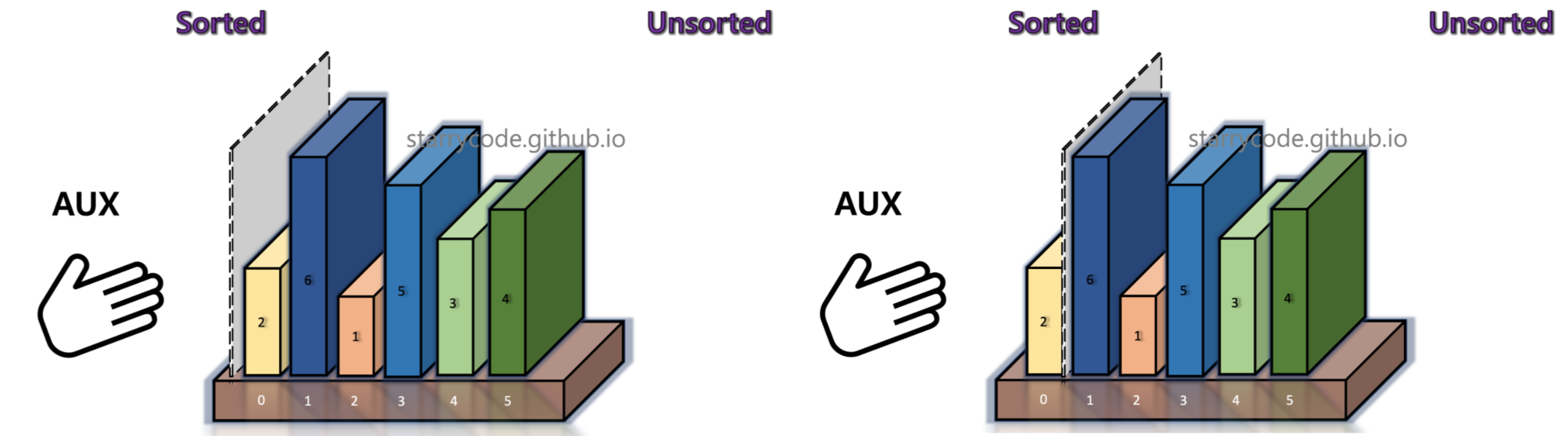
Figure 3: Insertion sort 1
2nd Iteration
We compare book 2 (left) and book 6 (right) adjacent to the grey divider. If left < right, which means that the books are already sorted, move the grey divider one index to the right. Anything on the left side of the divider is sorted. Anything on the right side of the divider is unsorted, and will be "inserted" into the appropriate index of the sorted sub-list.
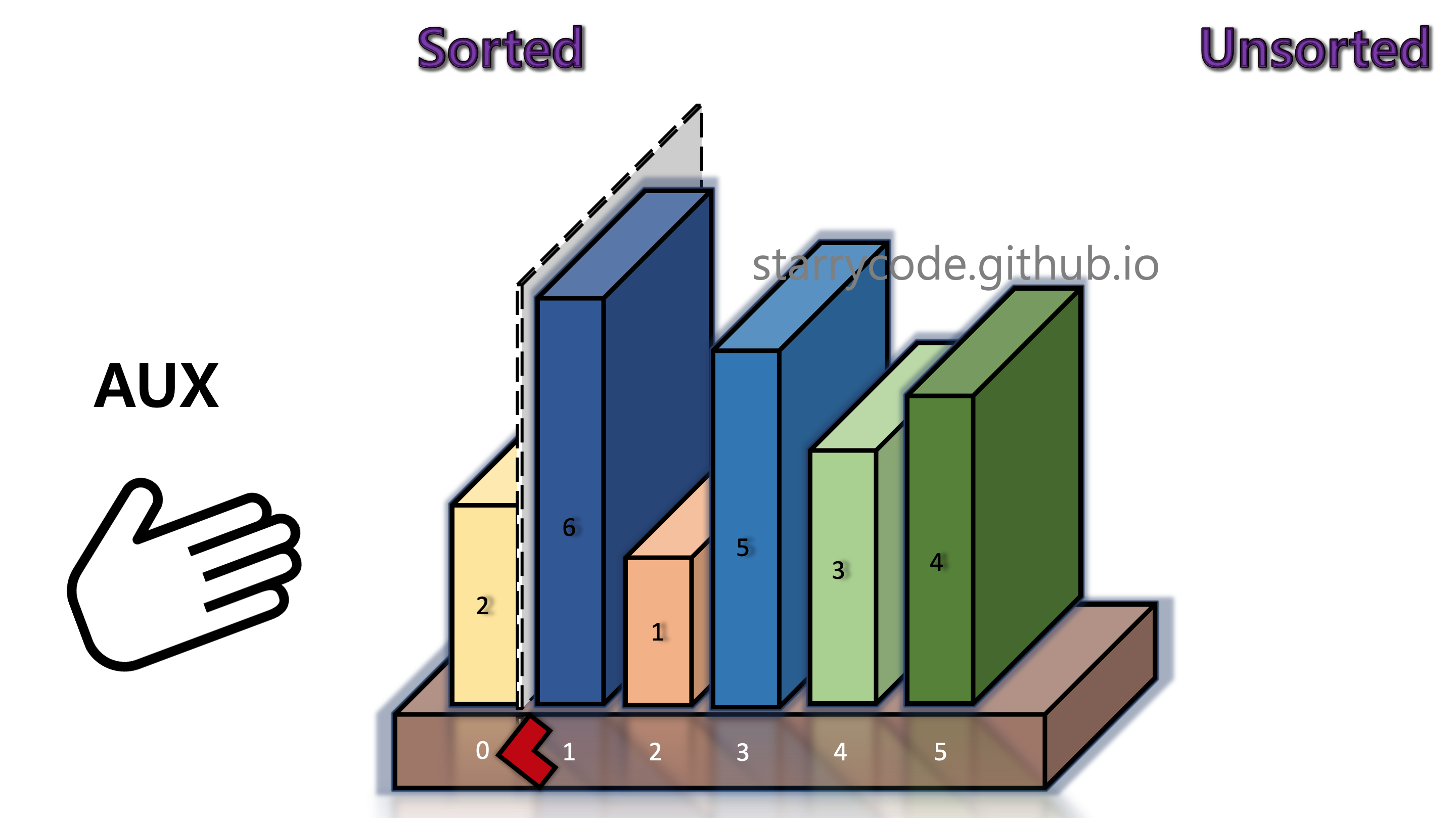
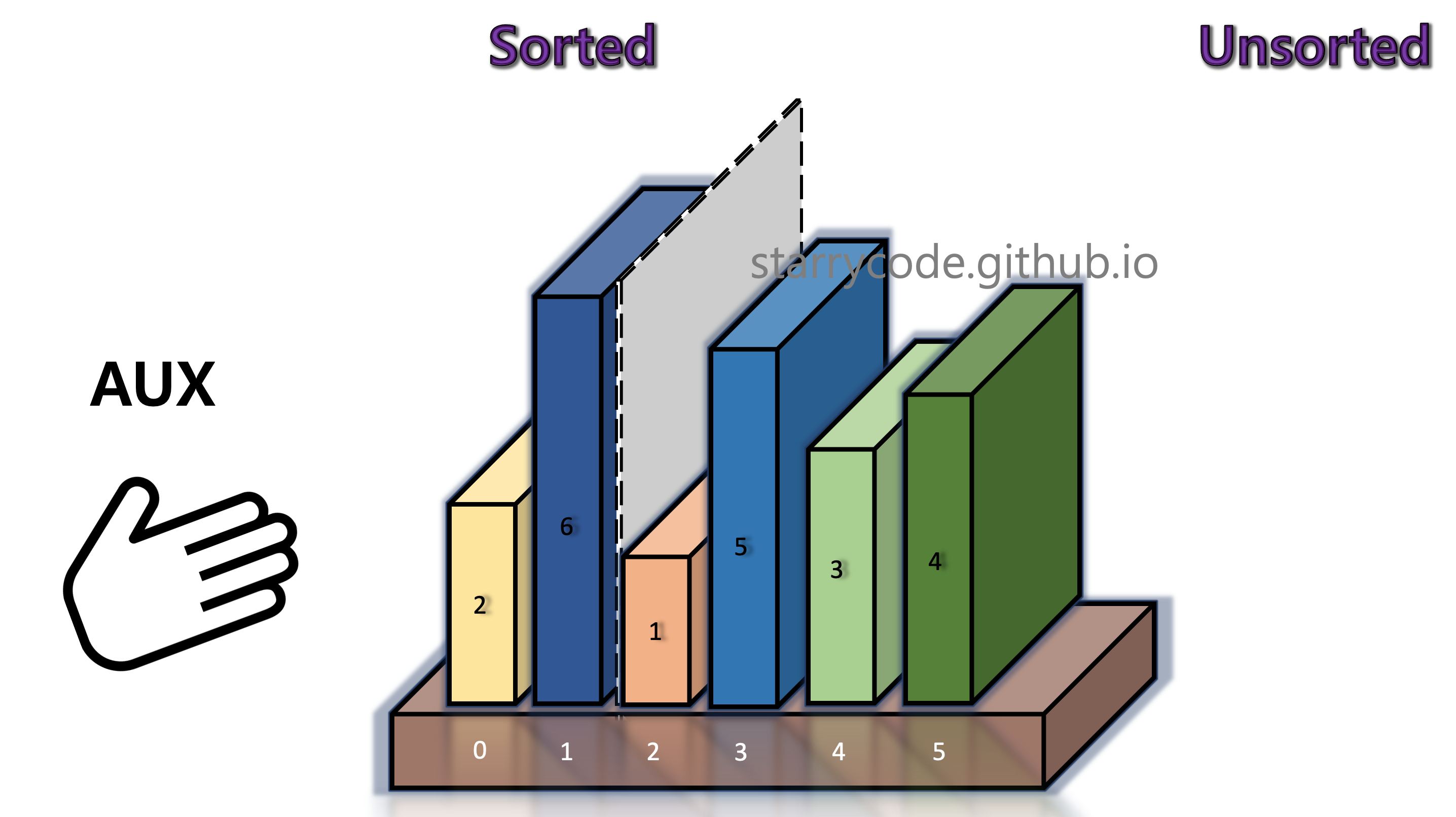
Figure 4: Insertion sort 2
3rd Iteration
We compare book 6 (left) and book 1 (right) adjacent to the grey divider. It turned out that the left item is greater than the right item. We take out the current unsorted item (right, book 1) and briefly keep it in the temporary storage (the hand icon), until it finds the appropriate index to be inserted.
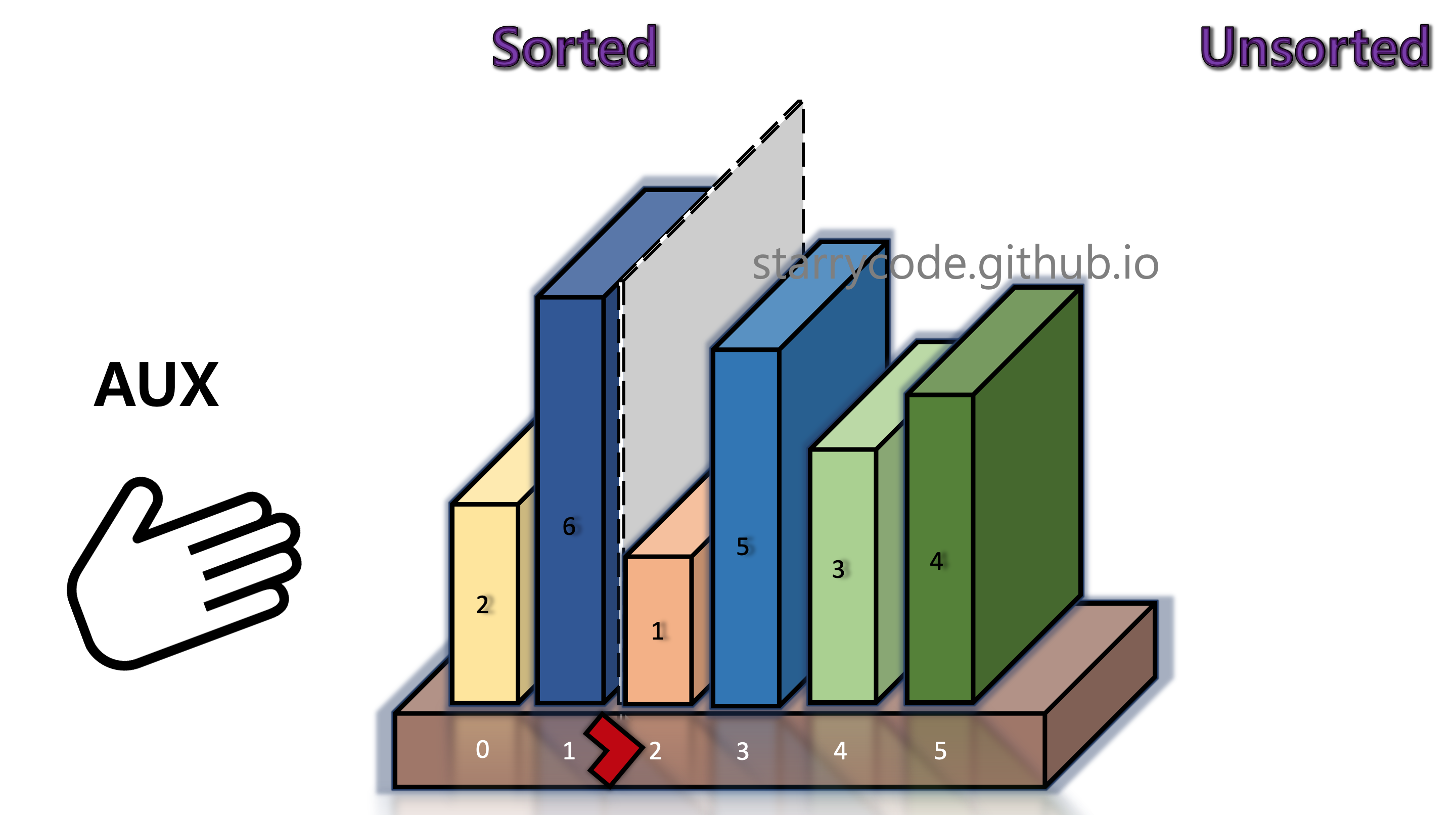
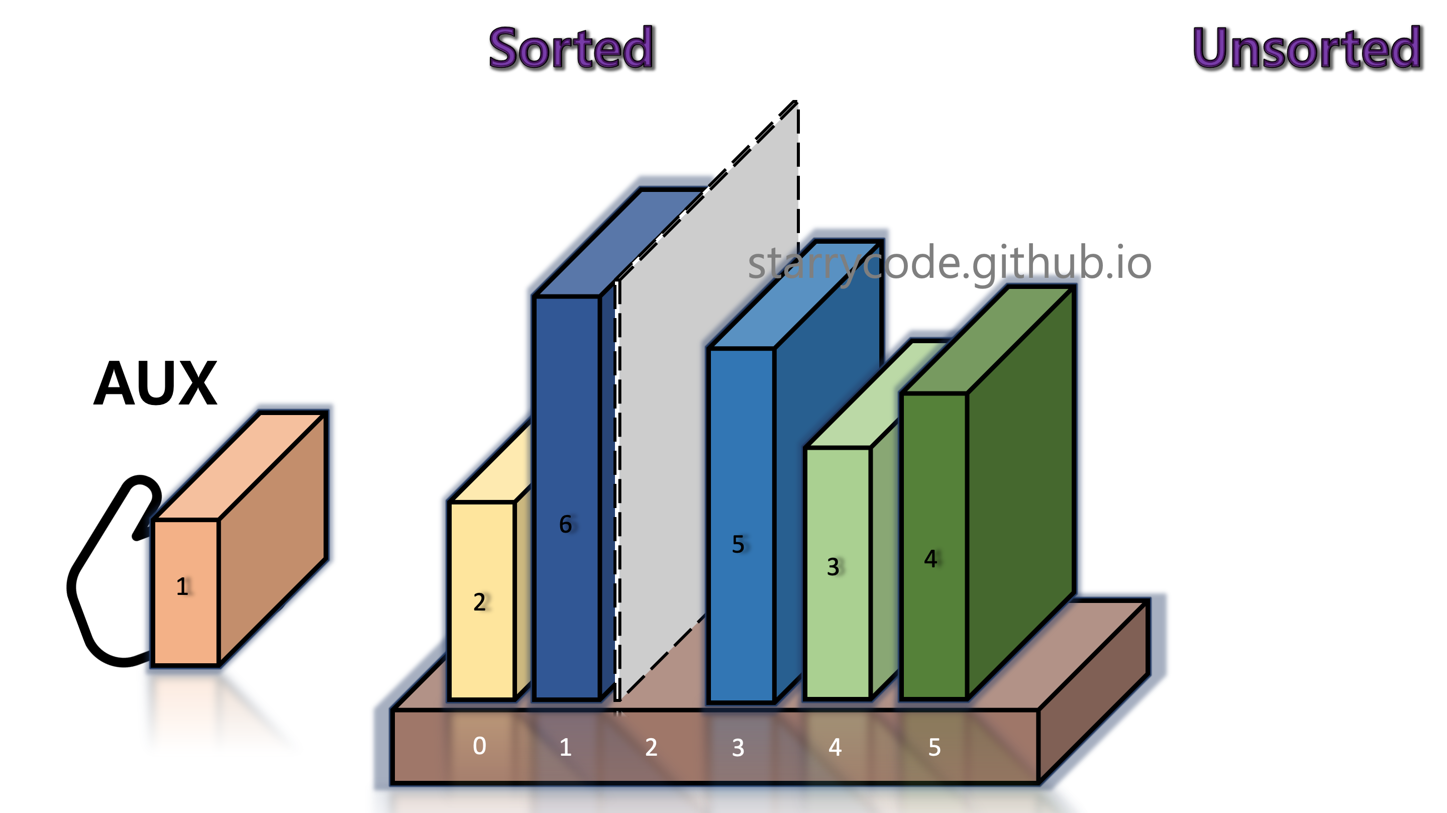
Figure 5: Insertion sort 3
The books on the left side of the divider shifts to the right, until the current block (book 1) in the temporary storage finds its right position.
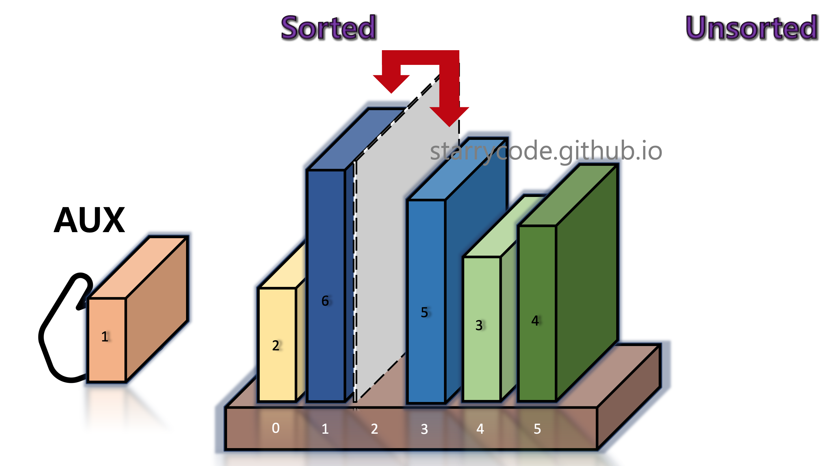
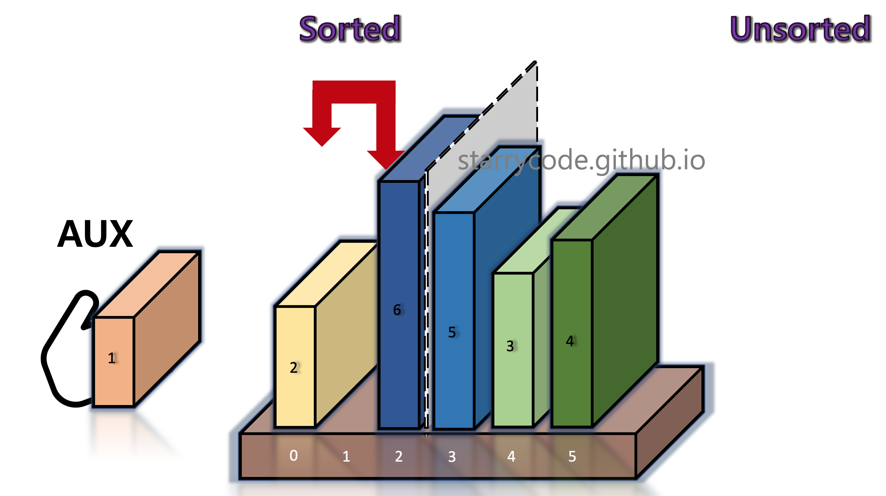
Figure 6: Insertion sort 4
Once the current block's (book 1's) appropriate index is found, the block is inserted into that index. Once the left side is sorted again, move the grey divider one index to the right.
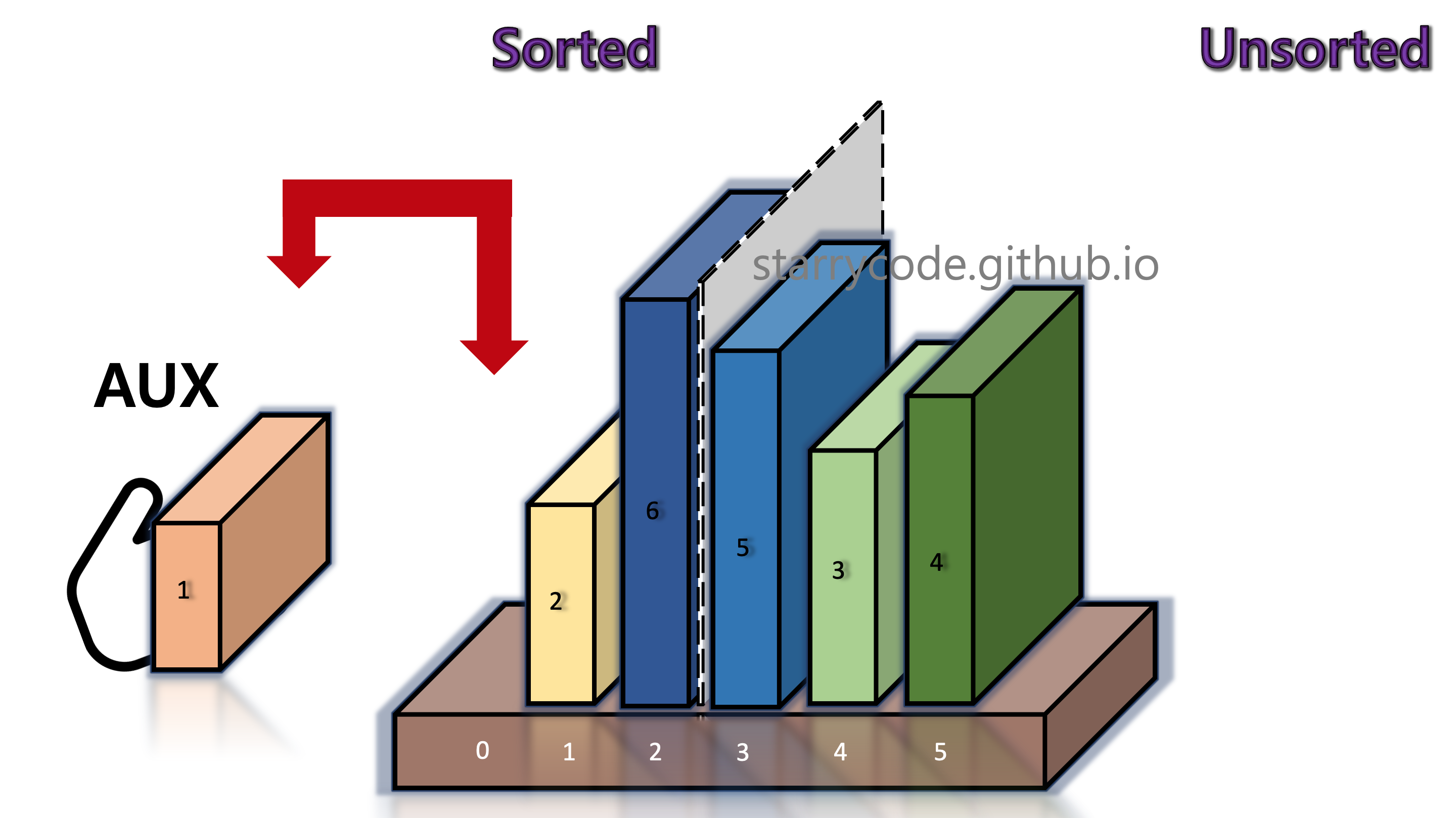

Figure 7: Insertion sort 5
4th Iteration
We repeat the same steps from above.
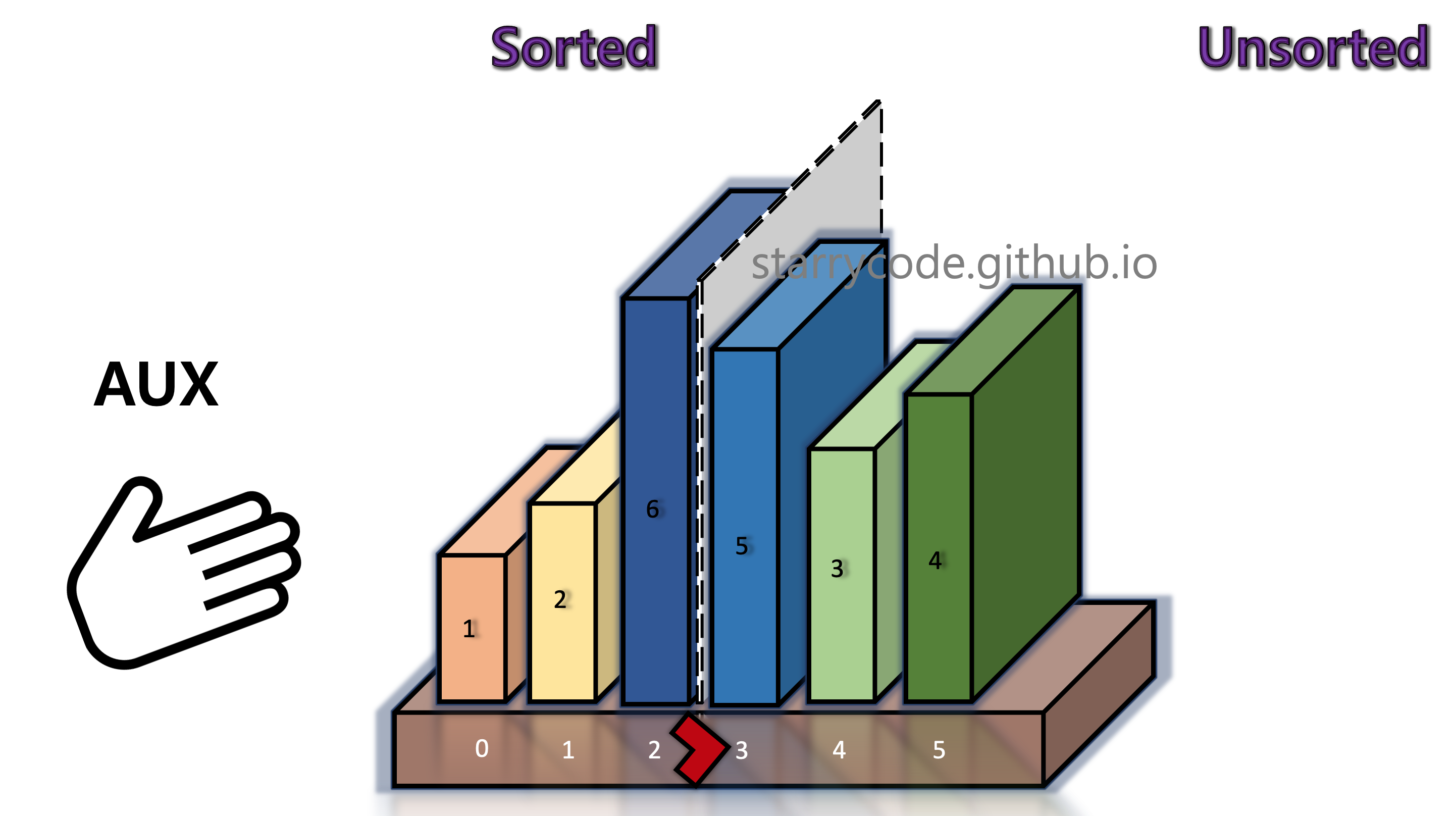
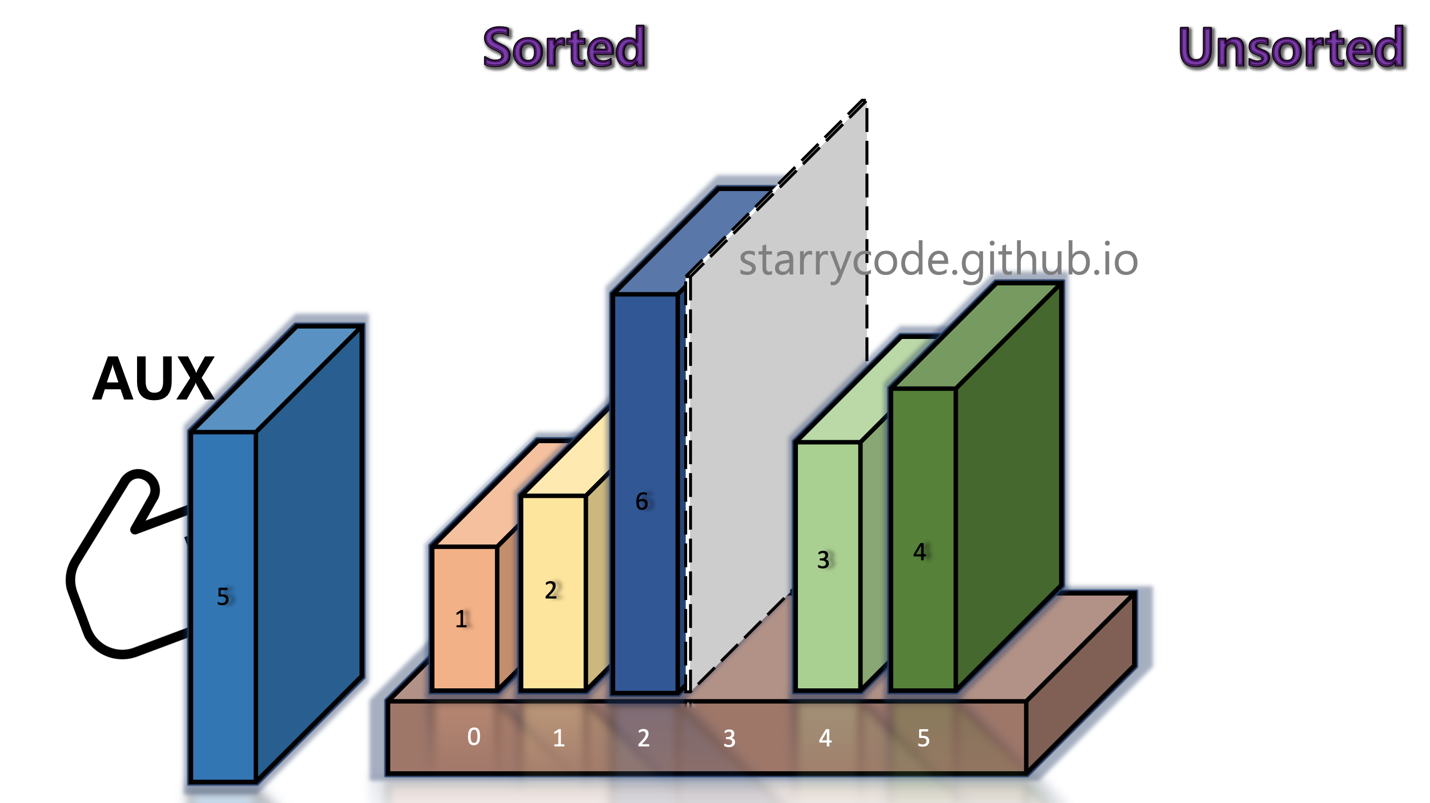
Figure 8: Insertion sort 6
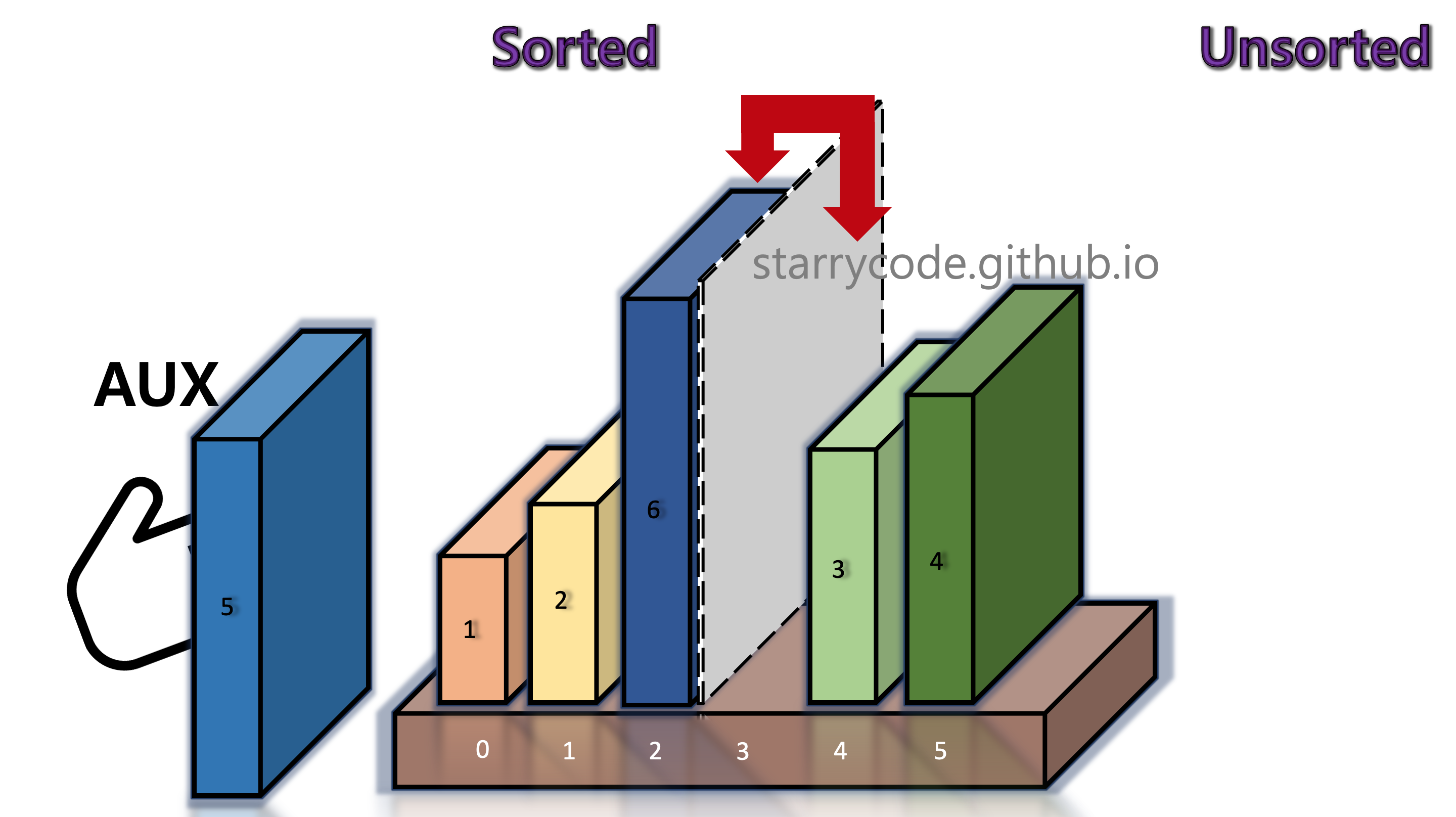
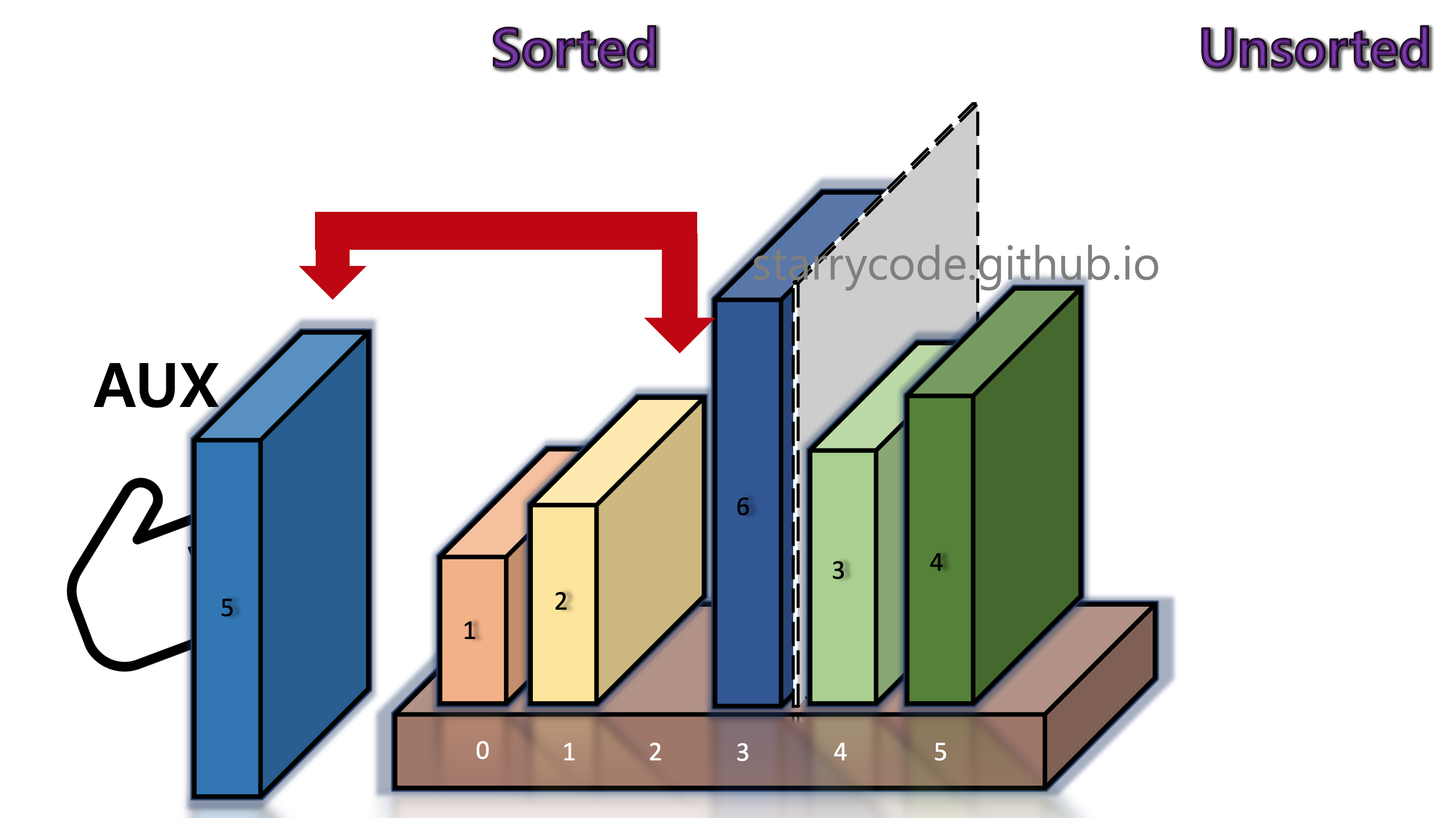
Figure 9: Insertion sort 7

Figure 10: Insertion sort 8
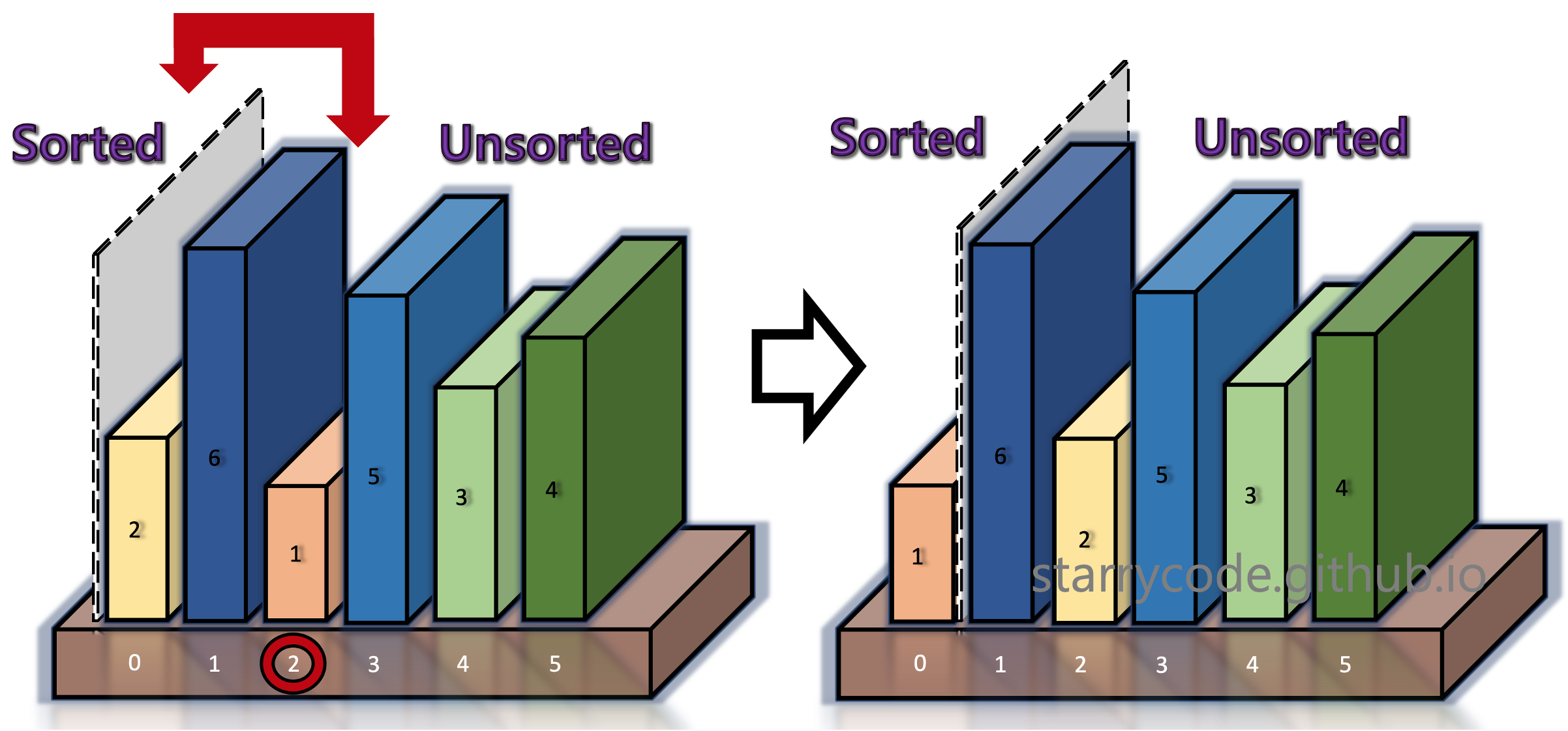
5th Iteration
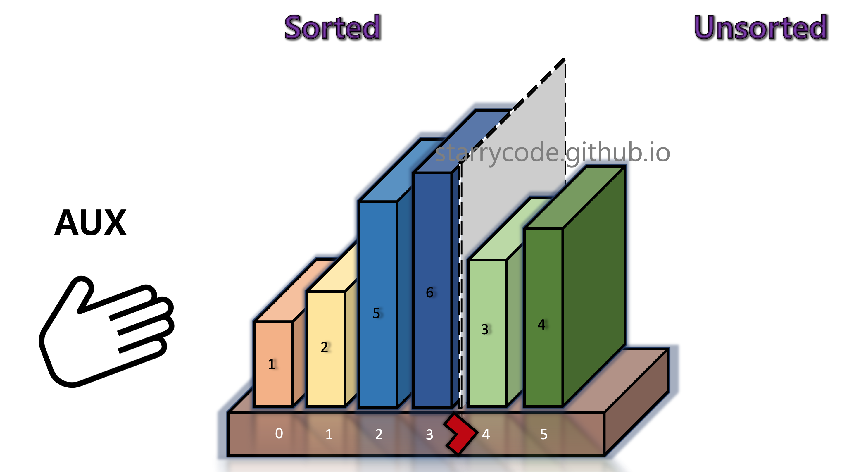
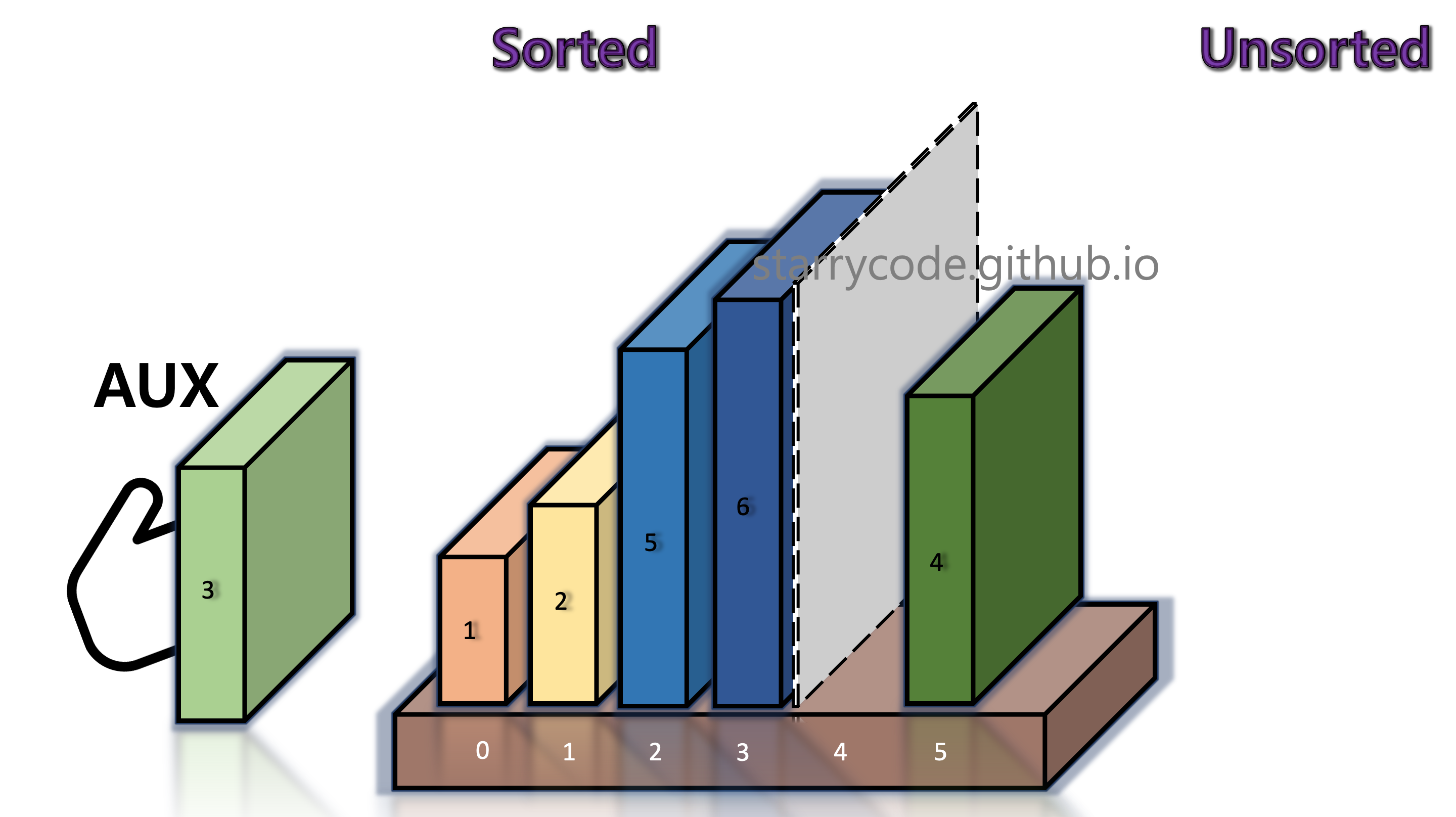
Figure 11: Insertion sort 9
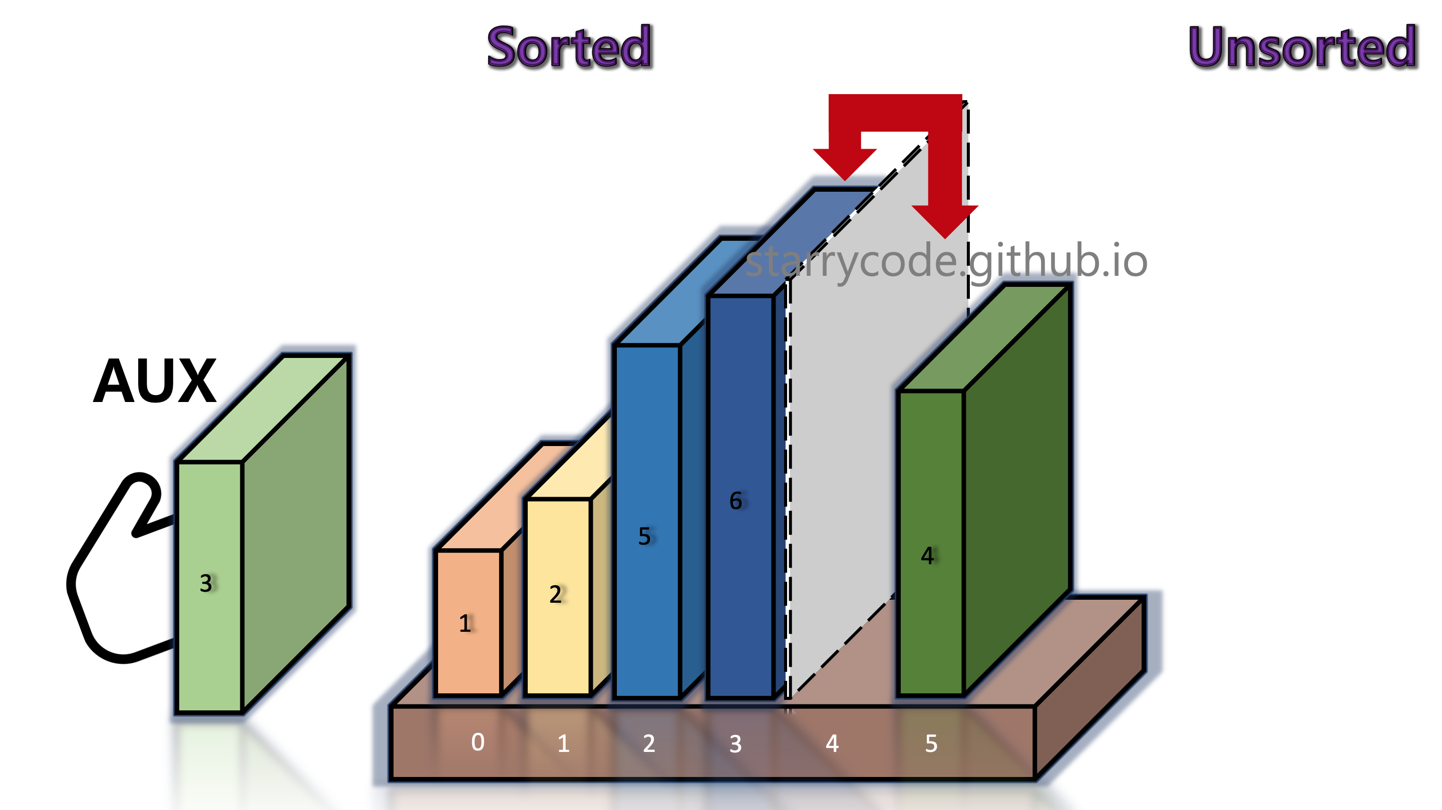
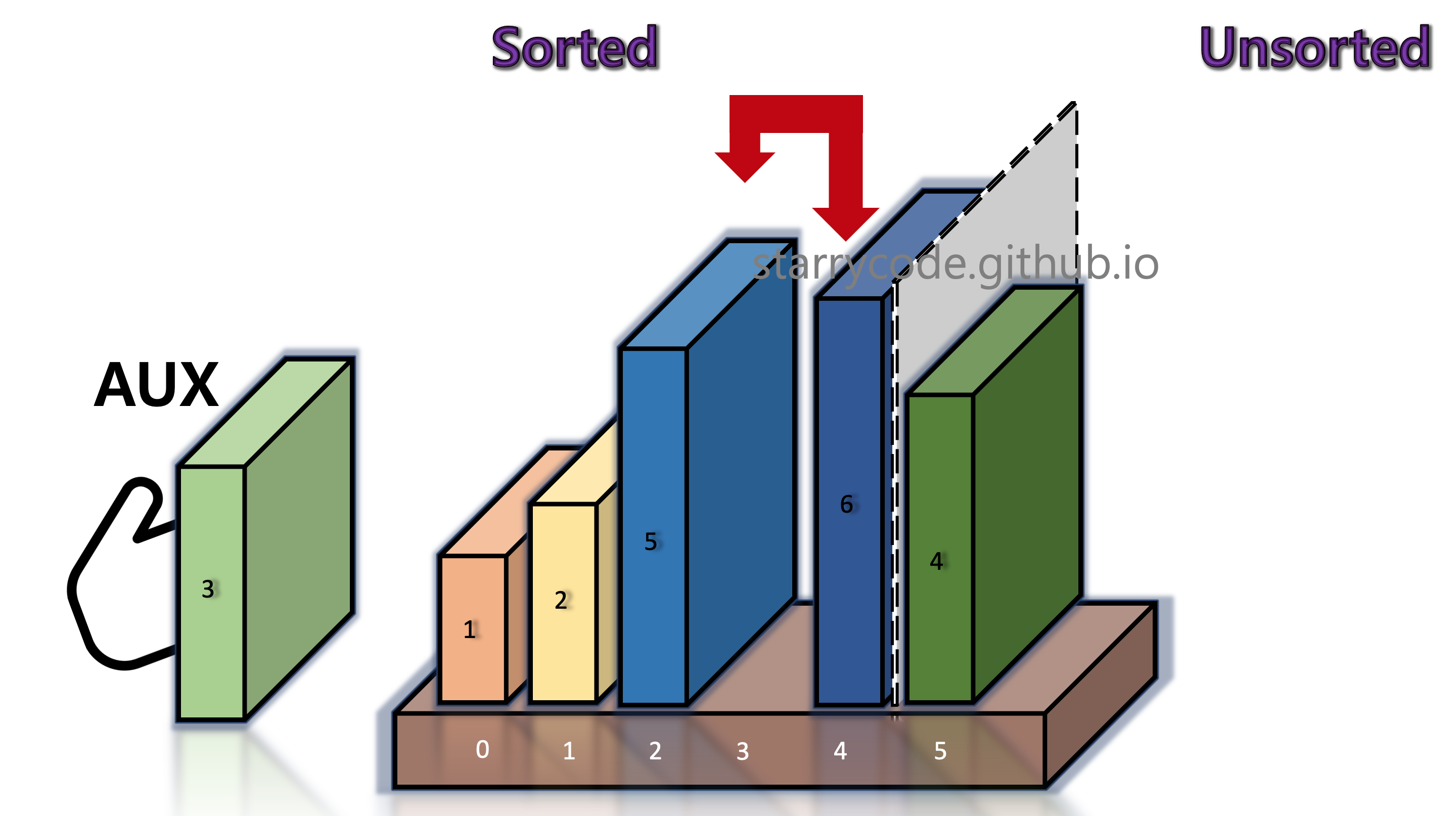
Figure 12: Insertion sort 10
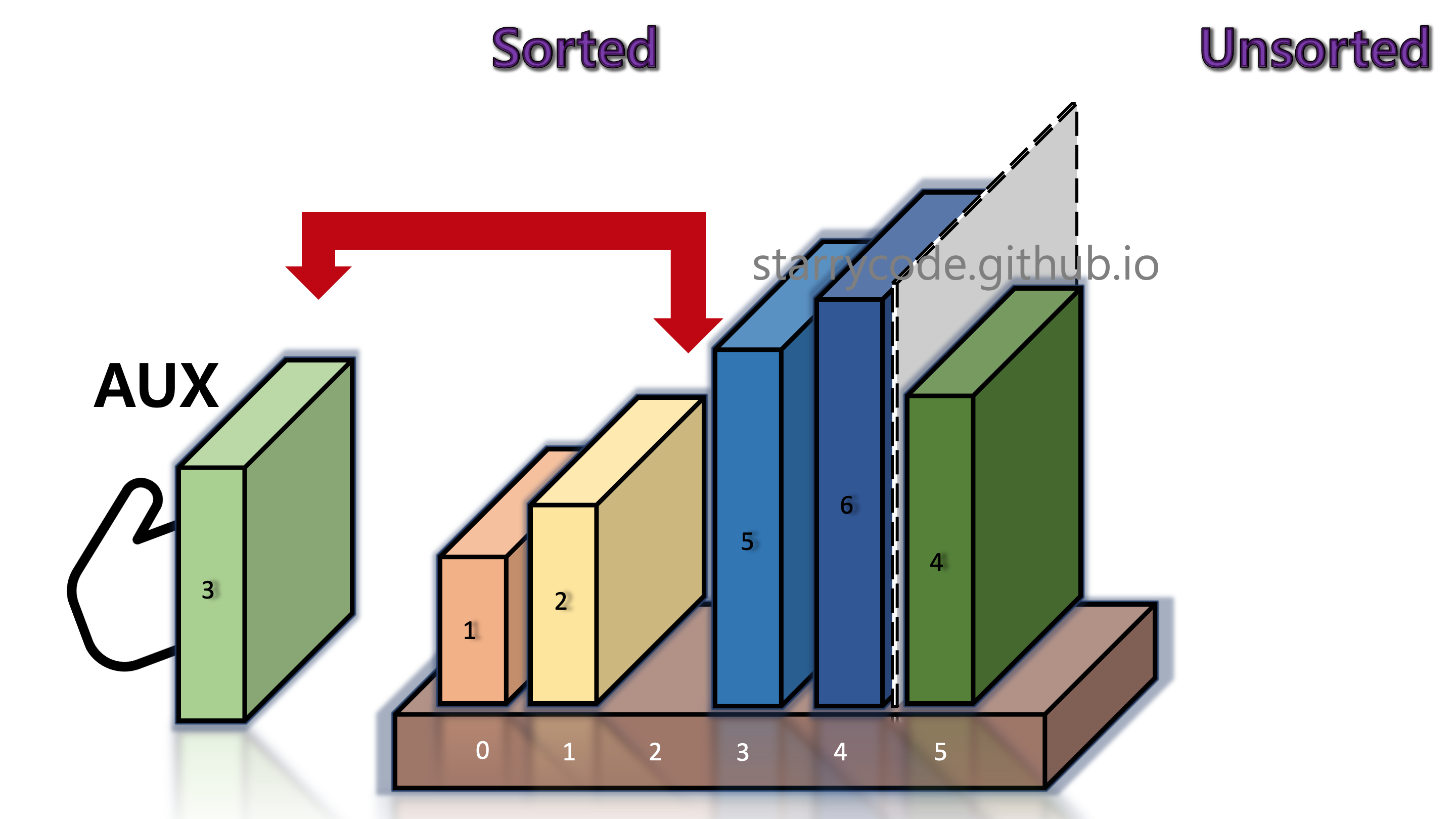
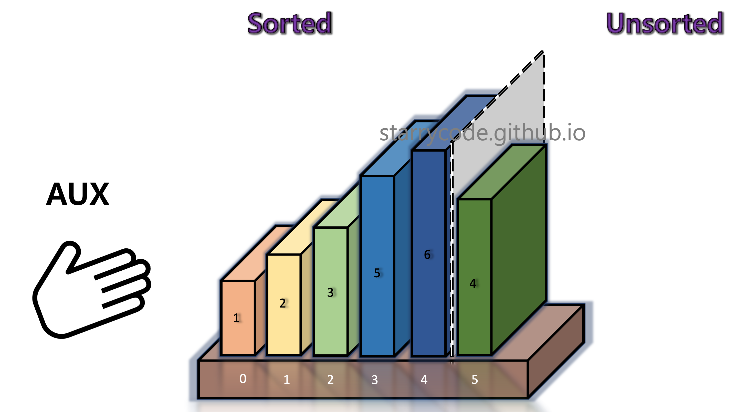
Figure 13: Insertion sort 11
6th Iteration
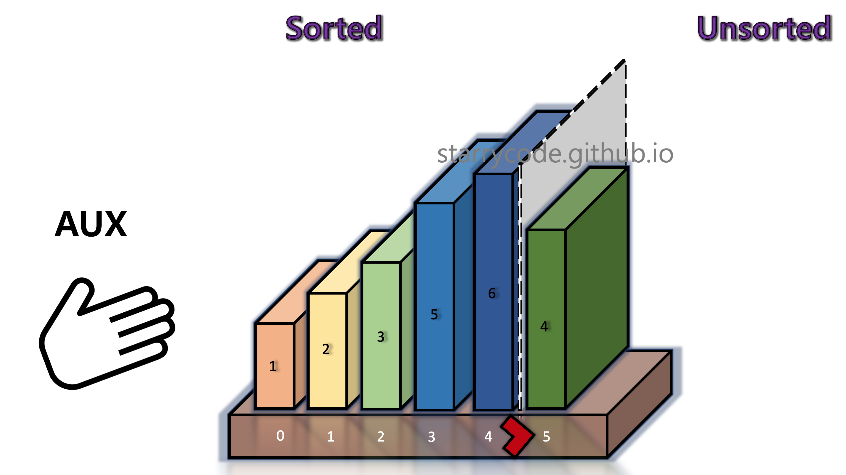
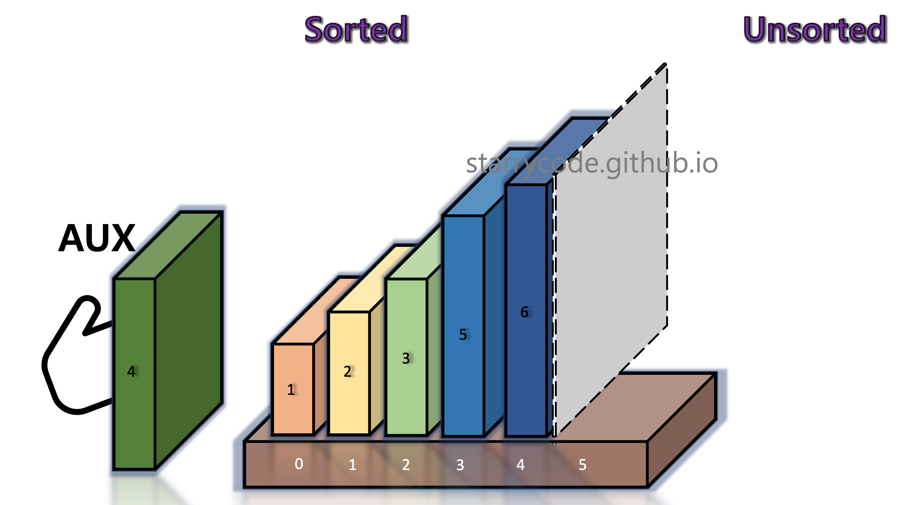
Figure 14: Insertion sort 12
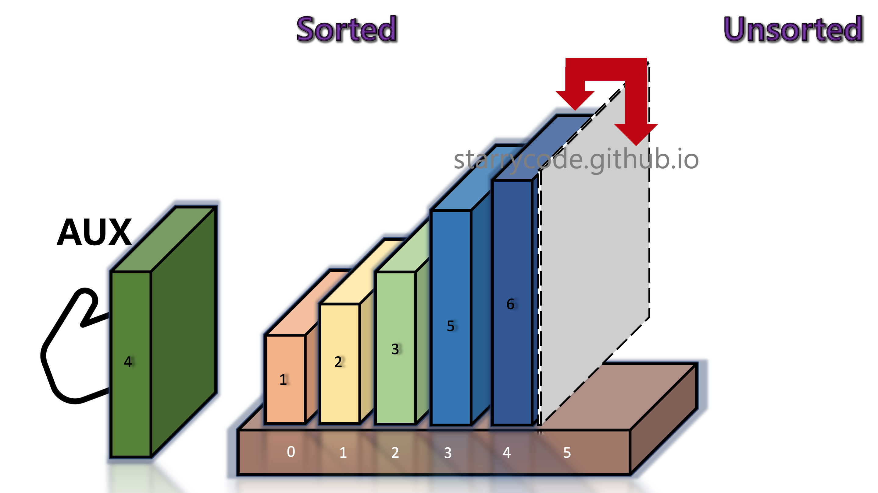
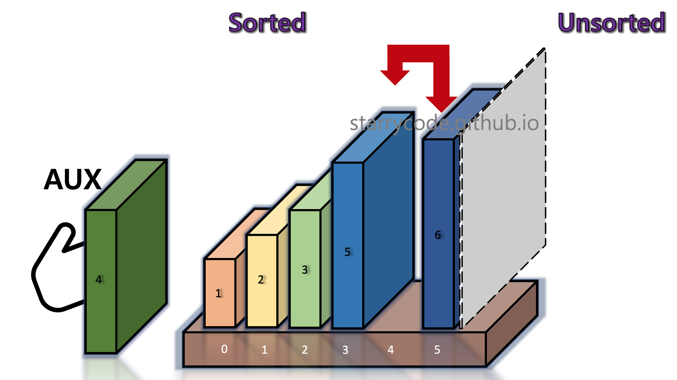
Figure 15: Insertion sort 13
The grey divider reached the end and the books are now sorted.
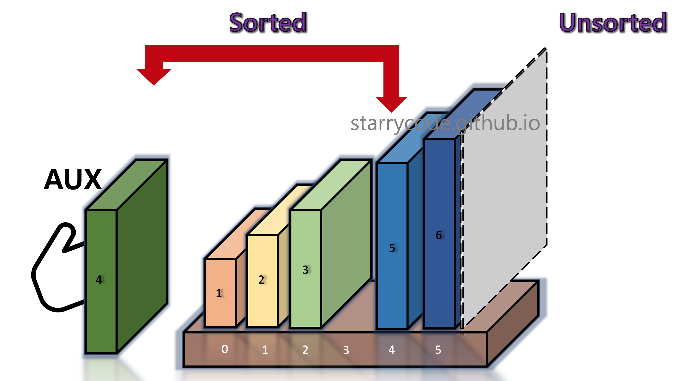
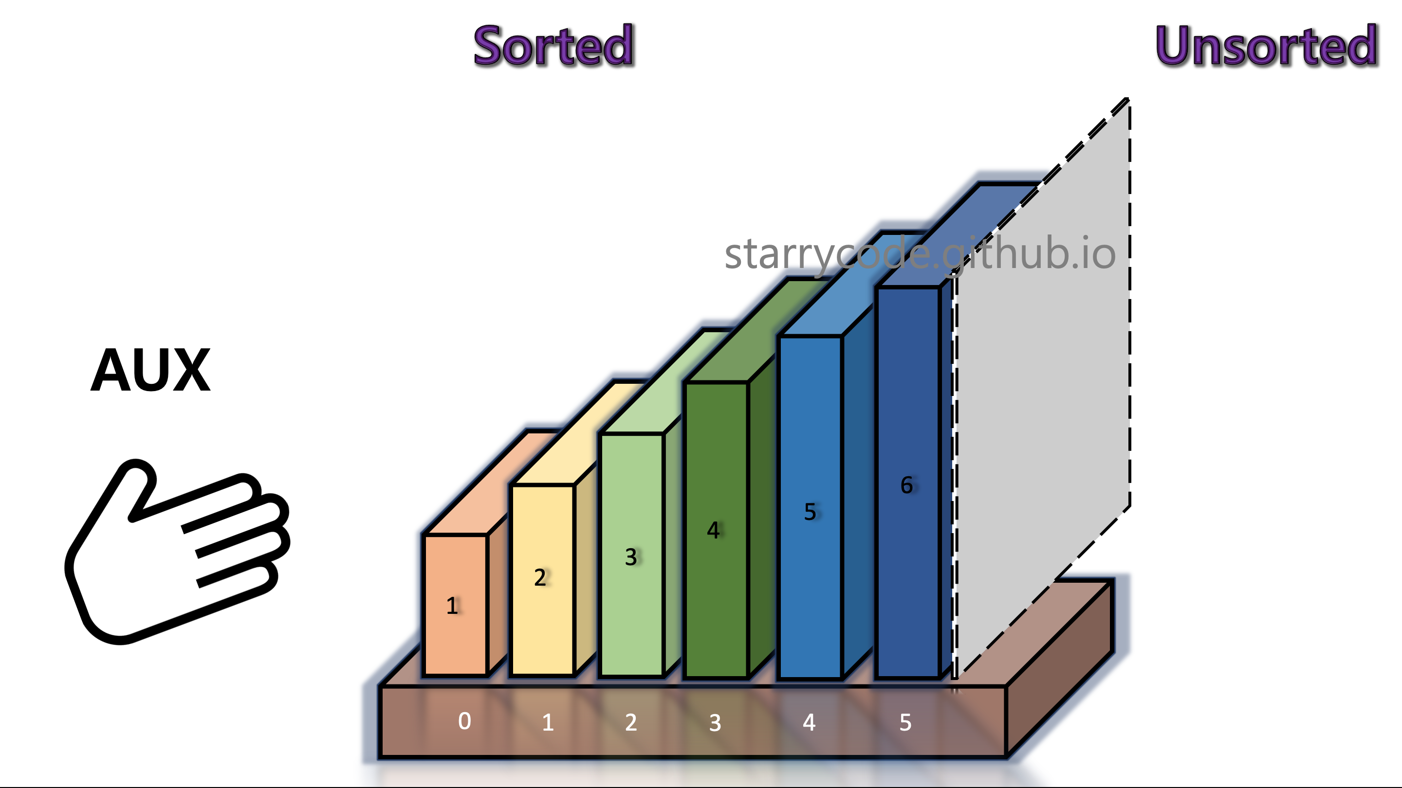
Figure 16: Insertion sort 14
Figure (17) is the gif represention of the insertion sort algorithm described above. Notice that the left side of the grey divider is a sorted sub-list, and right side of the divider is an unsorted sub-list. At the last iteration, the grey wall is at the end of the books, indicating the fact that all books are now sorted in an ascending order of sizes.
Figure 17: Insertion sort gif
1.2. Code Implementation
import java.util.Arrays;
//@author: Violet Oh

public class Insertion_Sort {
    public static void main(String[] args) {
        int[] array = {2, 6, 1, 5, 3, 4}; // The array we discussed.
        System.out.println(Arrays.toString(array));
        InsertionSort(array);
        System.out.println(Arrays.toString(array));
    }
    public static void InsertionSort(int[] array) {
        for(int i = 1; i < array.length; ++i)   // Starts from the second element.
        {
            int temp = array[i];    // Save the second element to another variable, "temp".

            int j;
            for(j = i; j > 0; --j)  // Shifts the elements until they are in order.
            {
                if(array[j-1] > temp)   // Checks if the first element is NOT SMALLER than the second element.
                {
                    array[j] = array[j-1];      // If so, the first element gets shifted to right (index + 1).
                }
                else
                {
                    break;  // If the first element is SMALLER than the second element already, nothing happens.
                }
            }
            array[j] = temp;    // The proper position for the element that was being compared with the element right before this.
            System.out.println(Arrays.toString(array)); // Print it out to see the changes.
        }
    }
}
Related Posts
Visual Understanding of Selection Sort Algorithm
Selection sort is an in-place comparison sorting algorithm. It has an $O(N^2)$ time complexity at all times. Effectively, the only reason that schools still teach selection sort is because it's an easy-to-understand, teachable technique, on the path to more complex and powerful algorithms.
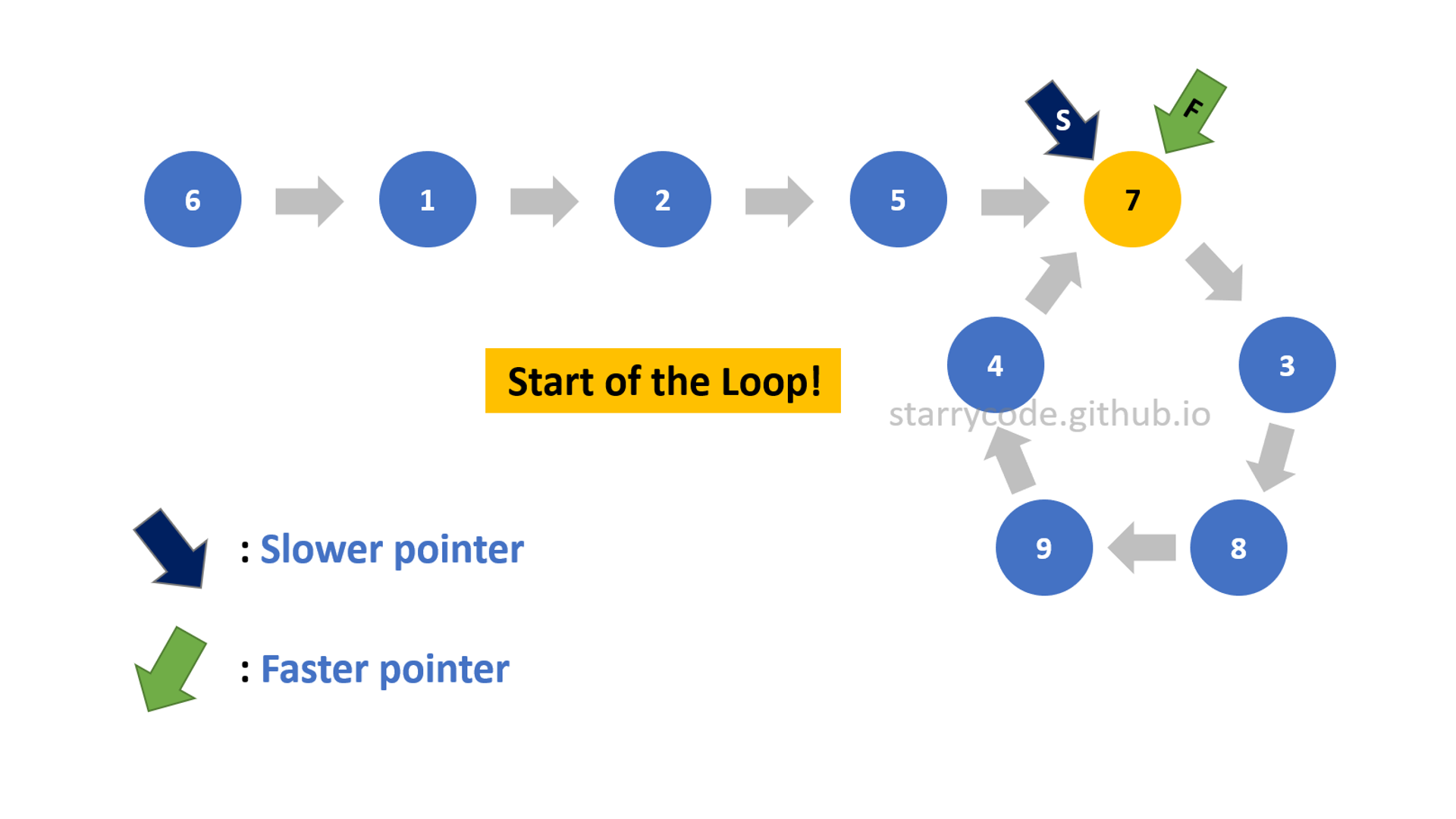
Detecting a Loop in Linked Lists and Finding a Start of the Loop
Linked List is a linear data structure where elements’ data part & address part are stored separately. Each node inside a linked list is linked using pointers and addresses. If there is a loop inside a linked list, how can it be detected? And if a loop is detected, how can the start of the loop be identified?