Detecting a Loop in Linked Lists and Finding a Start of the Loop

A Linked List is a linear data structure where, unlike the structure of an array, the elements’ data part and address part are stored separately. Each element inside a linked list is linked using pointers and addresses. Each element is called a node. Due to the structure of the linked list, an element cannot be accessed directly. However, the insertions and deletions of the linked list are far less complicated compared to those of the array. Therefore, preferences are given to using linked lists over arrays.

1. Linked List¶

A linked list would normally have a start and an end. The first node pointing to the second node, the second node pointing to the third node, etc. The last element in the linked list points to null, but nothing points to the first element in the linked list.

Figure 1: Typical linked list

1.1. Detecting a Loop¶

How about when there’s a loop inside a list? In this post, detecting a loop inside a list, and detecting the start of the loop will be discussed. Consider the following linked list in Figure (2).

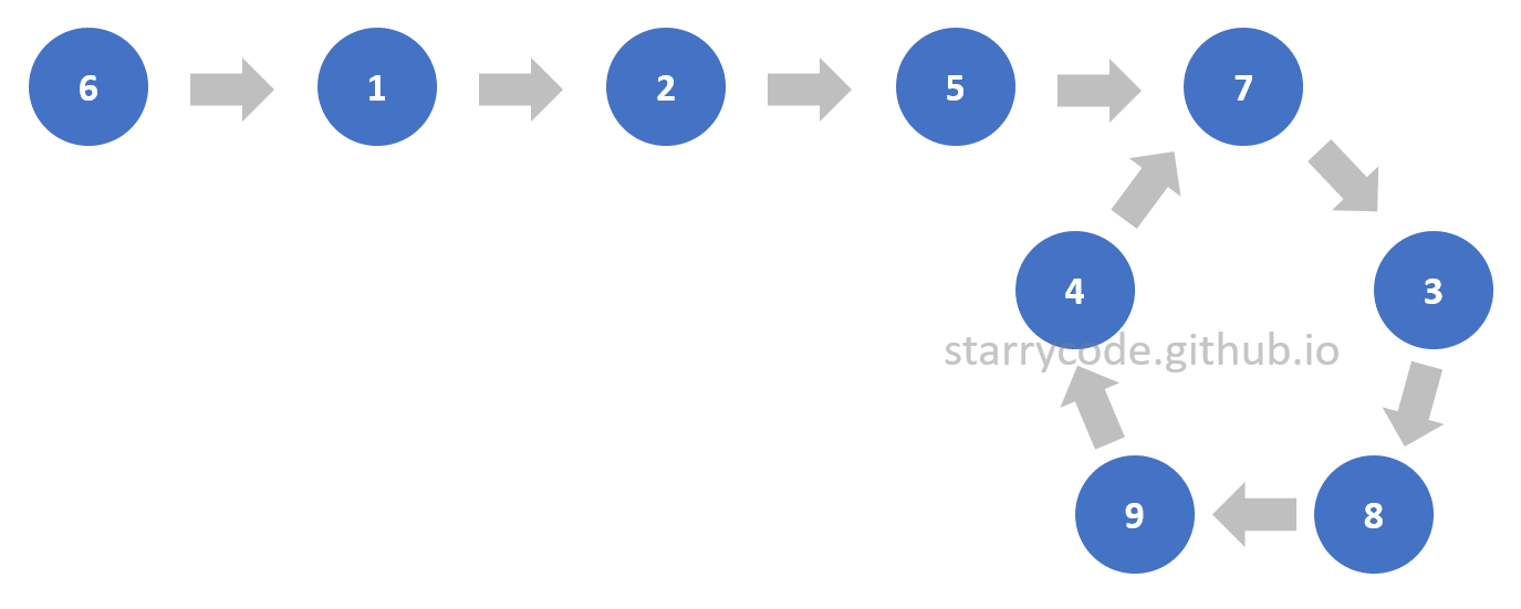
Figure 2: Linked list with a loop

Detecting a loop inside a linked list is the first step. There are two pointers: a slower pointer ‘S’ and a faster pointer ‘F’ will be used to detect a loop.

The slower pointer will be moving one node at a time whereas the faster pointer will be moving two nodes at a time. A linked list without a loop would never have two pointers pointing to the same node since the faster pointer is always ahead of slower pointer and the distance between the two pointers will always be increasing every time the pointers move. This is Floyd’s Cycle-finding algorithm, and it is also called the “tortoise and the hare algorithm”. (The faster pointer is a hare, and the slower pointer is a tortoise.) Therefore, if the two pointers wind up pointing to the same node, it implies that there is a loop inside a list.

This is the strategy to detect a loop inside a list. The following is the illustration of the two pointers moving and winding up pointing to the same node.

Detecting a Loop Illustration

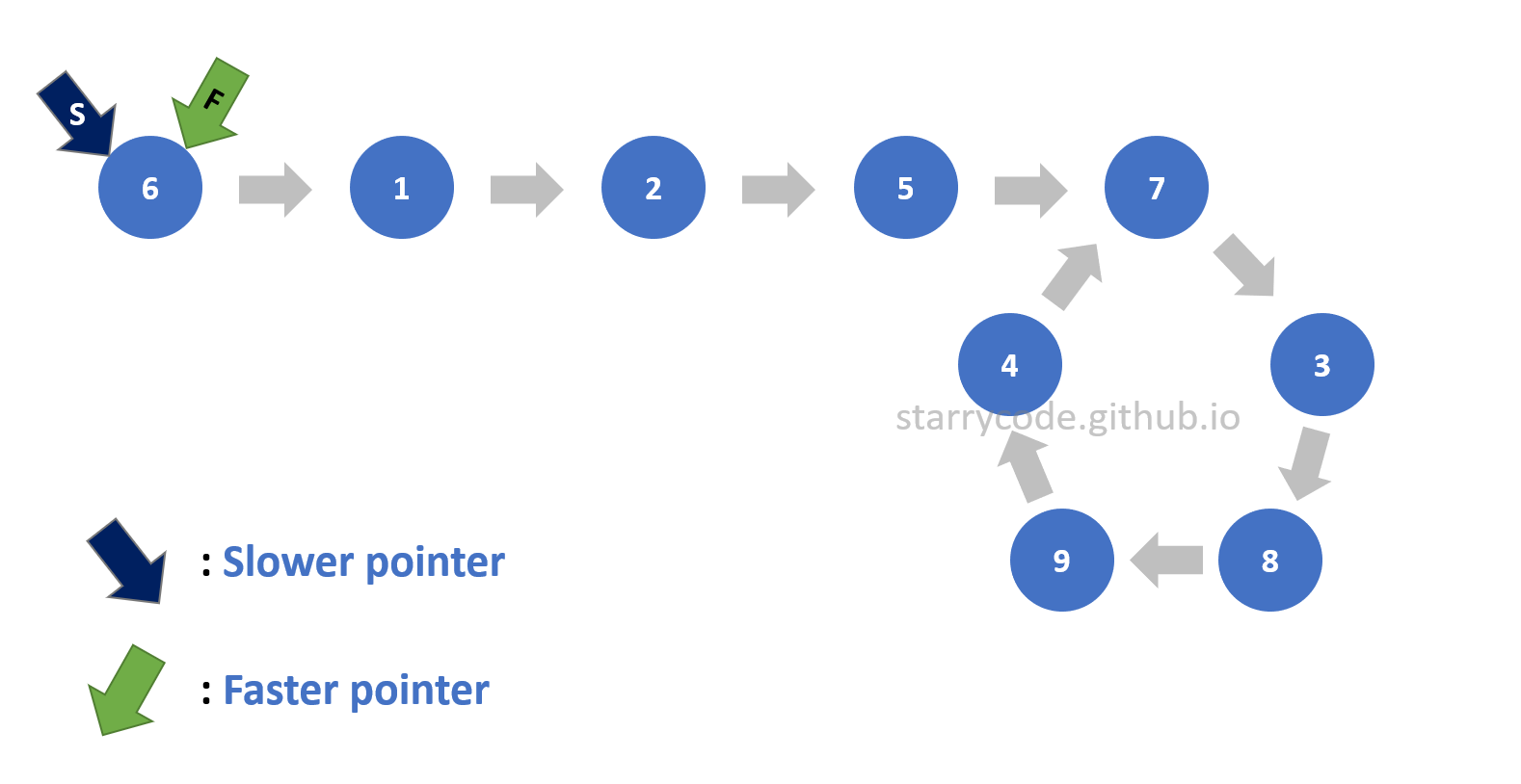
Figure 3: Loop detection 1

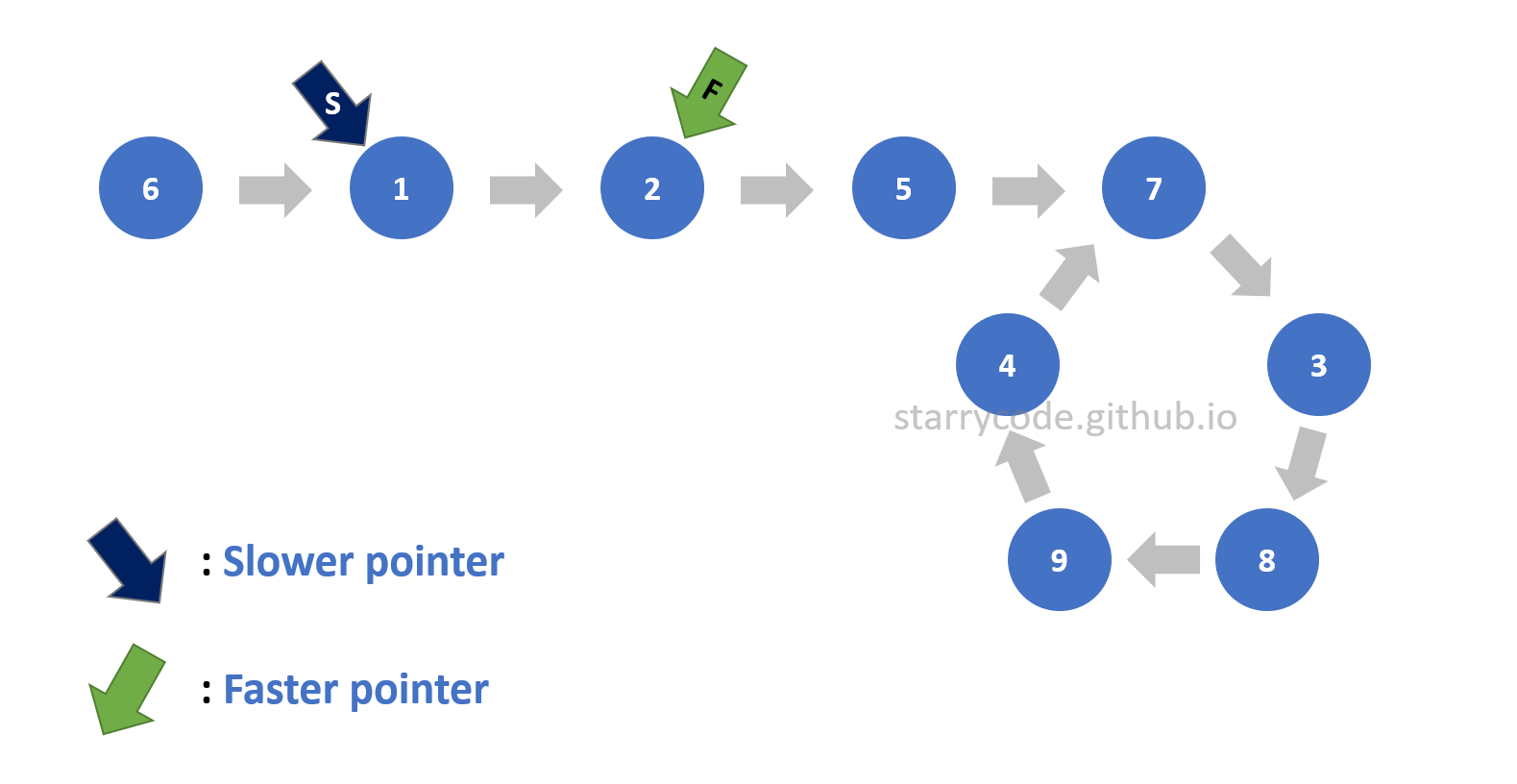
Figure 4: Loop detection 2

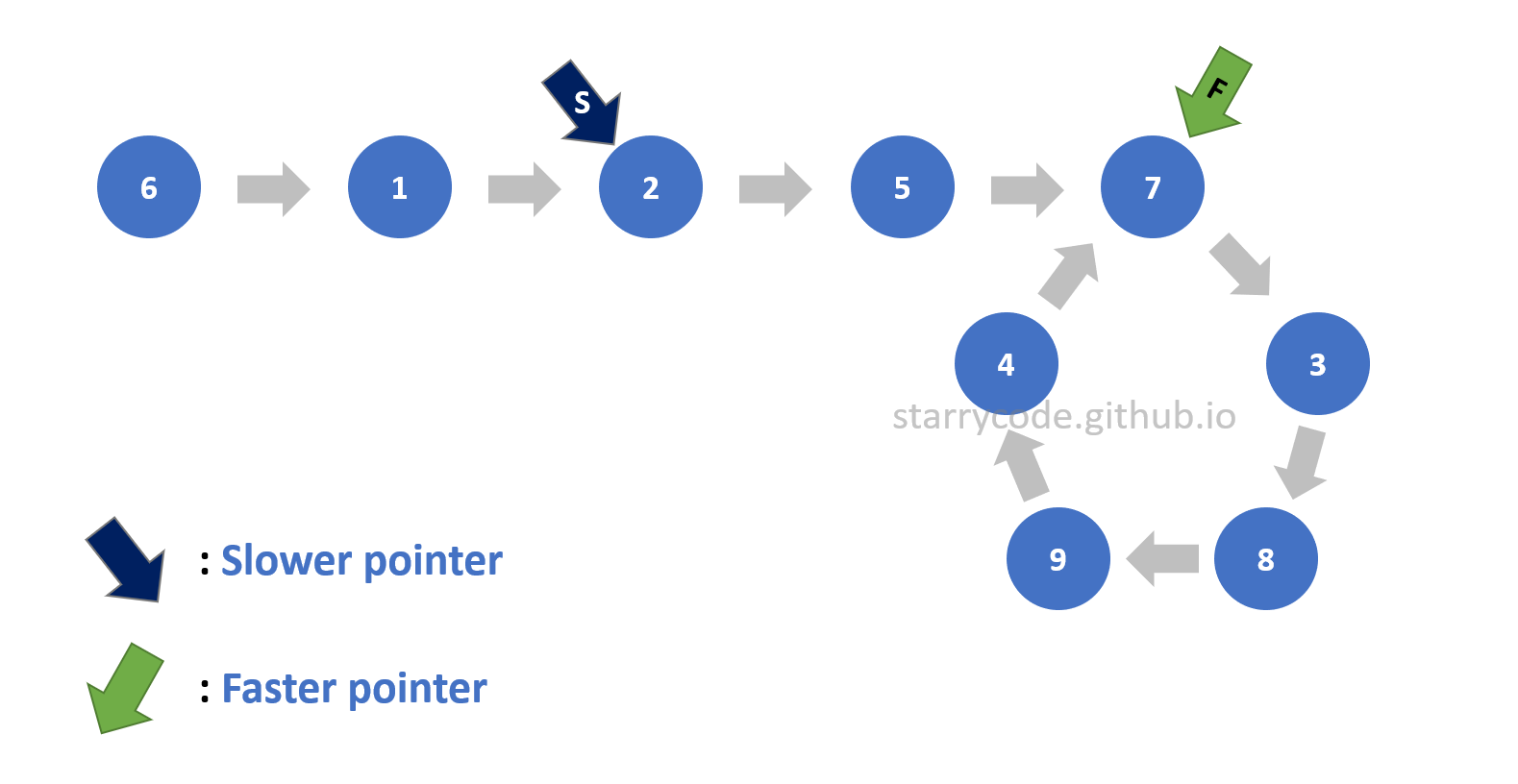
Figure 5: Loop detection 3

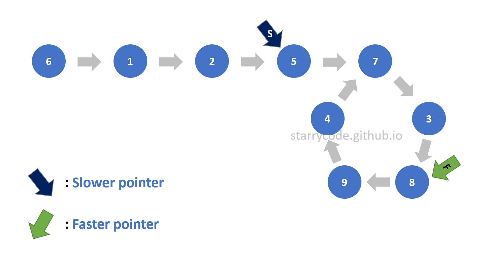
Figure 6: Loop detection 4

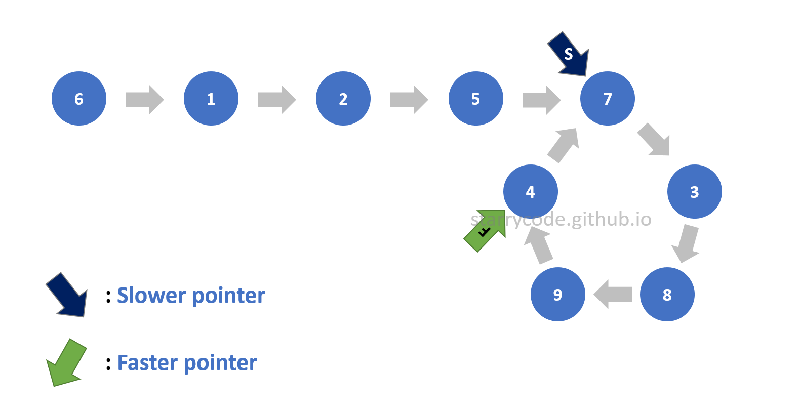
Figure 7: Loop detection 5

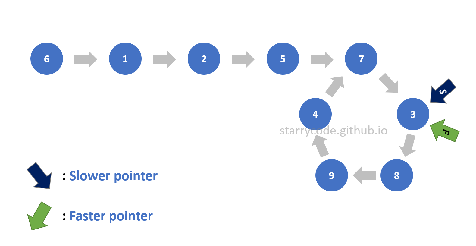
Figure 8: Loop detection 6

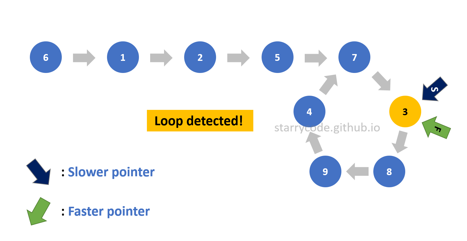
Figure 9: Loop detection 7

Figure (10) is the gif represention of the Floyd's Cycle-finding algorithm described above. Note that the faster pointer moves two nodes at a time whereas the slower pointer moves one node at a time. You can see that both pointers pointed to the node 3, which implies that this linked list has a loop inside itself.

Figure 10: Loop detection gif

1.2. Finding the Start of the Loop¶

The next step is to figure out the start of the loop. For this step, the faster pointer stays pointing at the same node continuing from the previous step, and the slower pointer points to the starting node of the list. Then both pointers move one node at a time until they meet. Once the pointers meet or point to the same node, then that particular node is the start of the loop.

Finding the start of the Loop Illustration

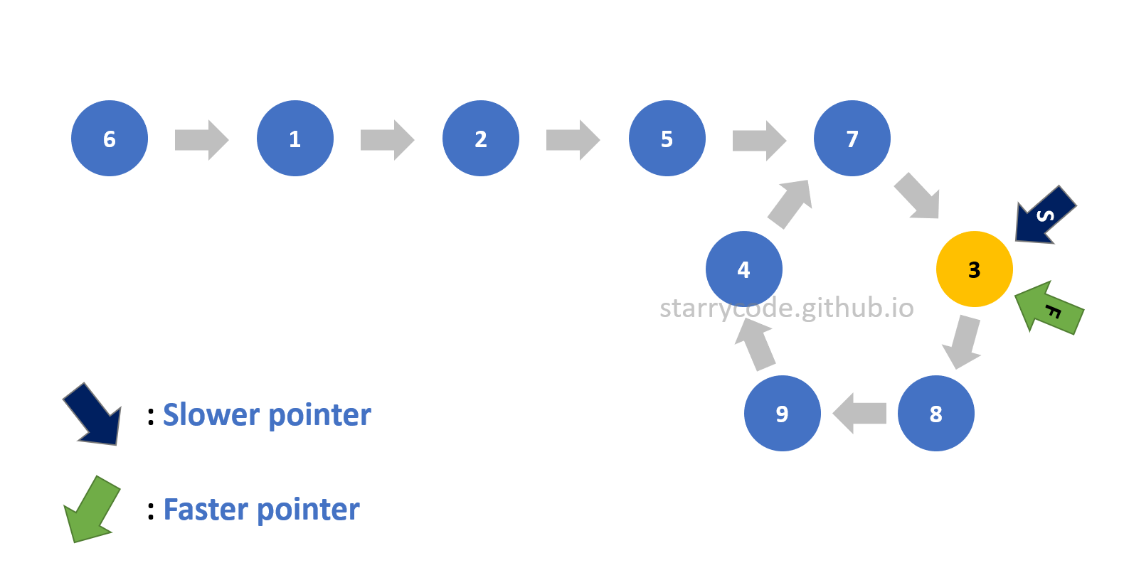
Figure 11: Finding start 1

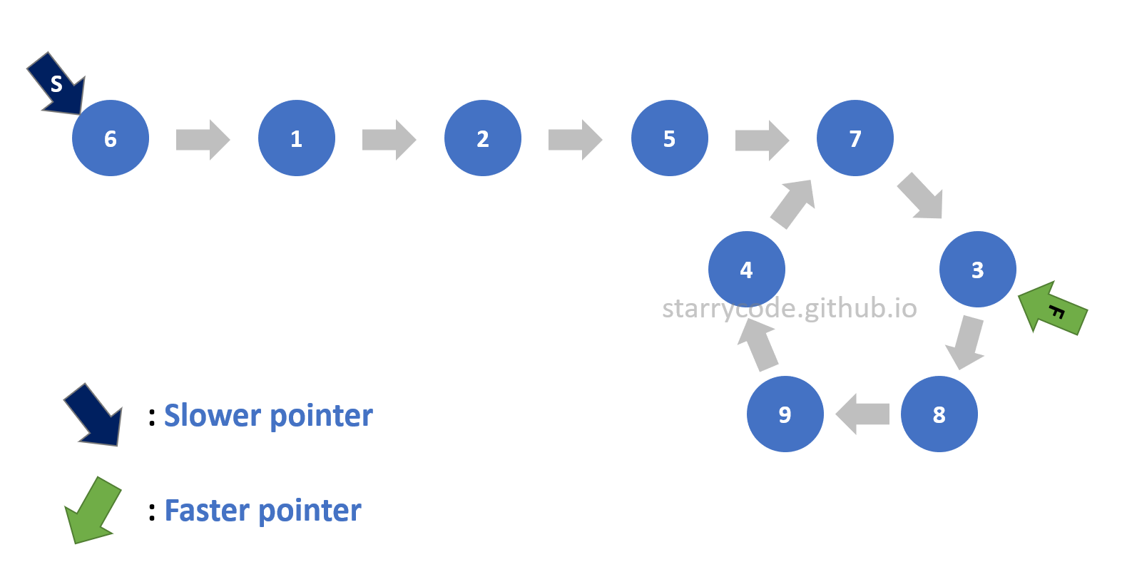
Figure 12: Finding start 2

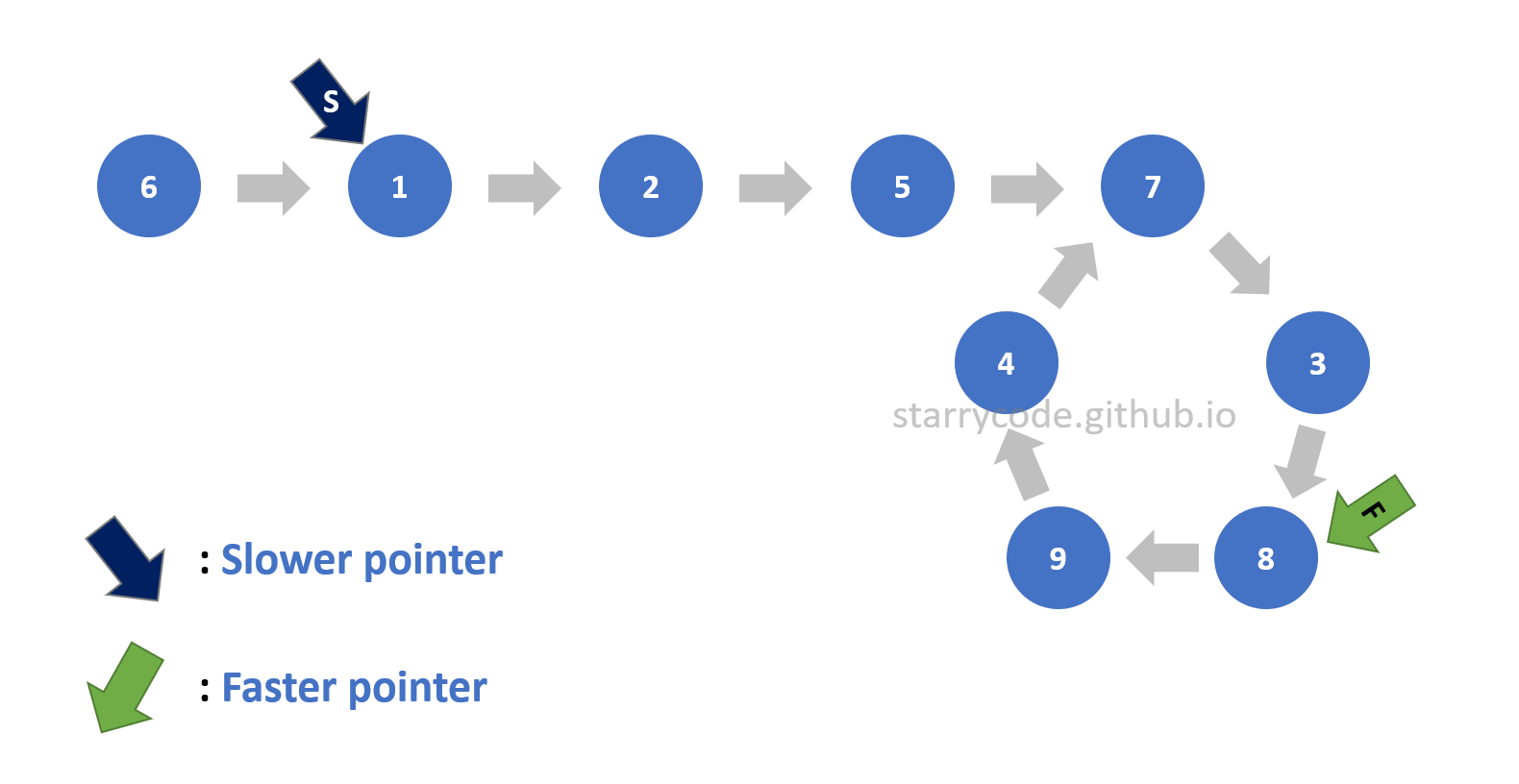
Figure 13: Finding start 3

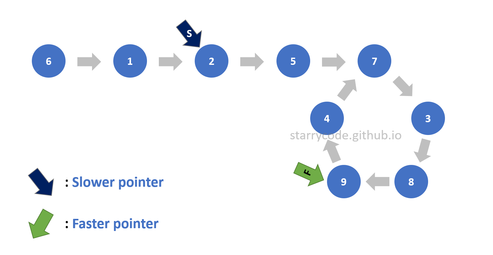
Figure 14: Finding start 4

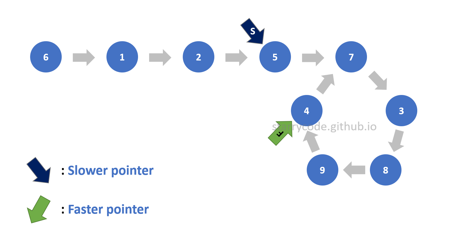
Figure 15: Finding start 5

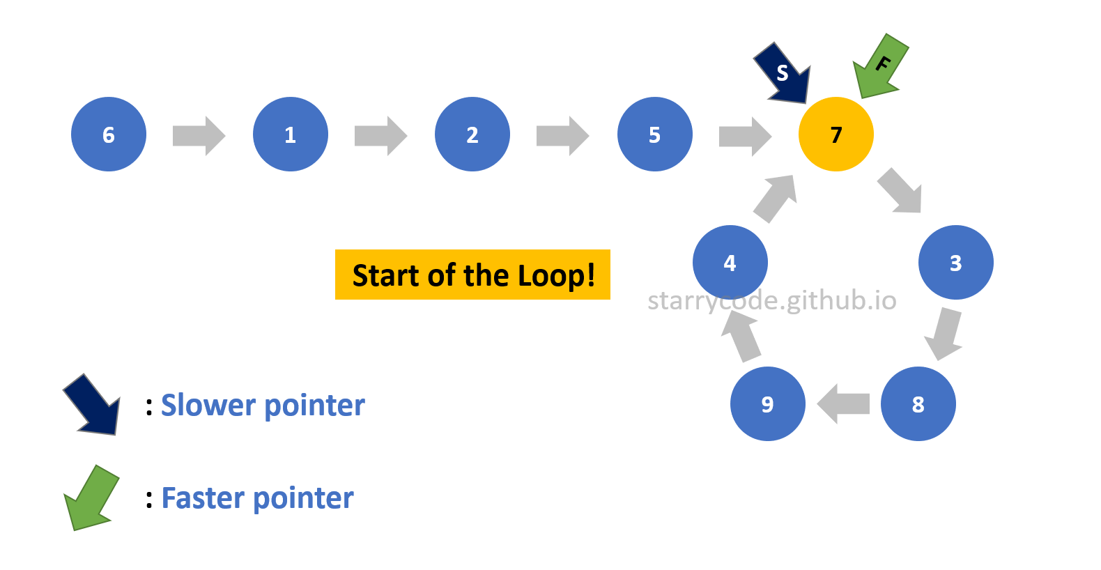
Figure 16: Finding start 6

Figure (17) is the gif represention of finding the start of the loop as described above. Note that the faster pointer stays at the same node from Figure (9) and the slower pointer starts from the very first node of the list. Both of the pointers move one node at a time and they meet at the start of the loop.

Figure 17: Finding start gif

1.3. Algorithm Explanation¶

How does this algorithm work? Let l be the length of the loop, and m be the distance between the start of the loop and the very first node of the list.

l and m Illustration

In the following diagram, l is 5 since 5 nodes are forming a loop and m is 4 since the distance between node 6 and node 7 is 4.

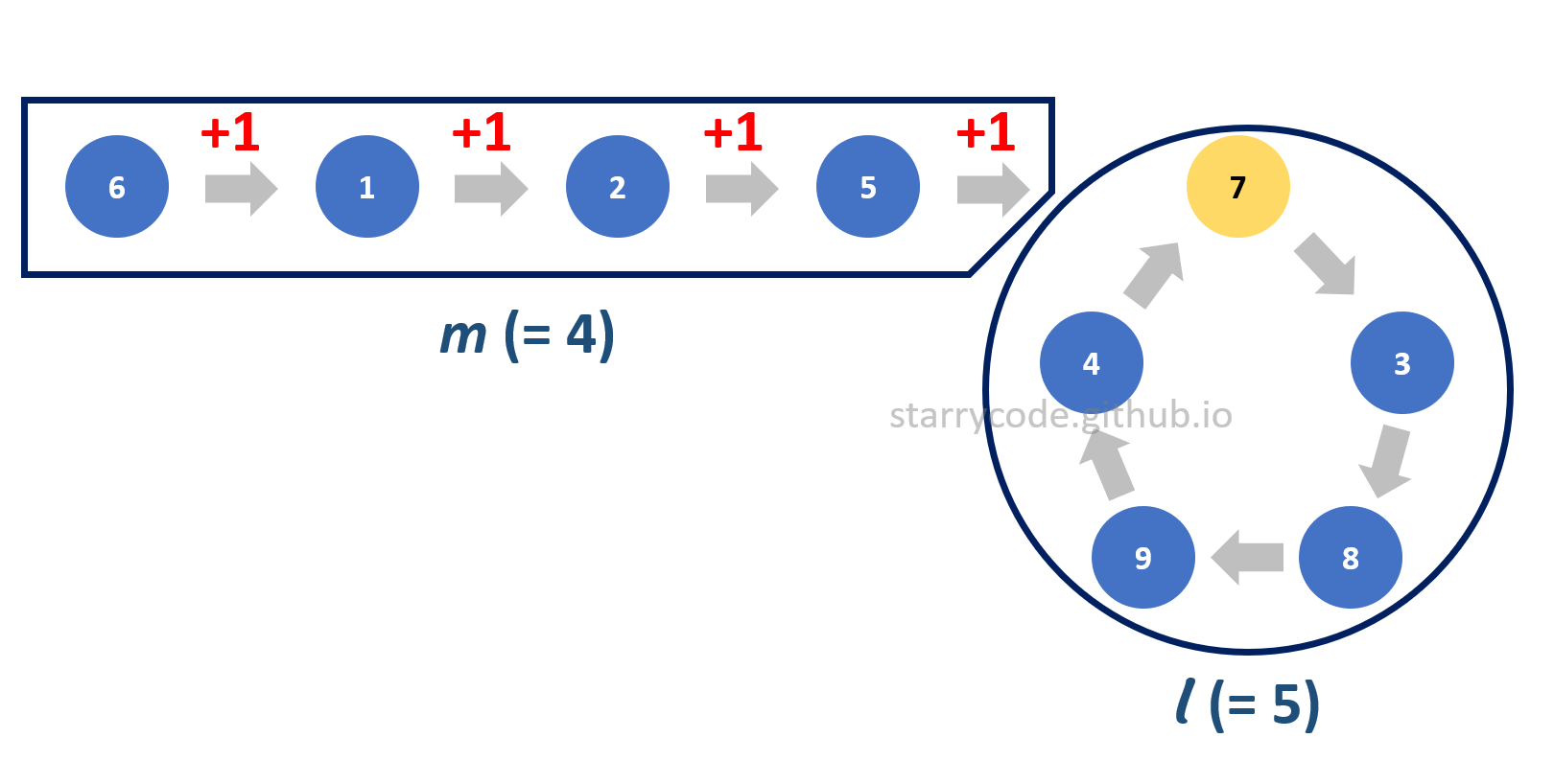
Figure 18: Algorithm explanation 1

k Illustration

Let k be the distance between the start of the loop and the node that was pointed by both pointers while detecting the loop. Recall that in the first step (Floyd’s cycle-finding algorithm), both pointers met at the node 3. Therefore, in the following diagram, k is 1 since the distance between the node 7 and the node 3 is 1.

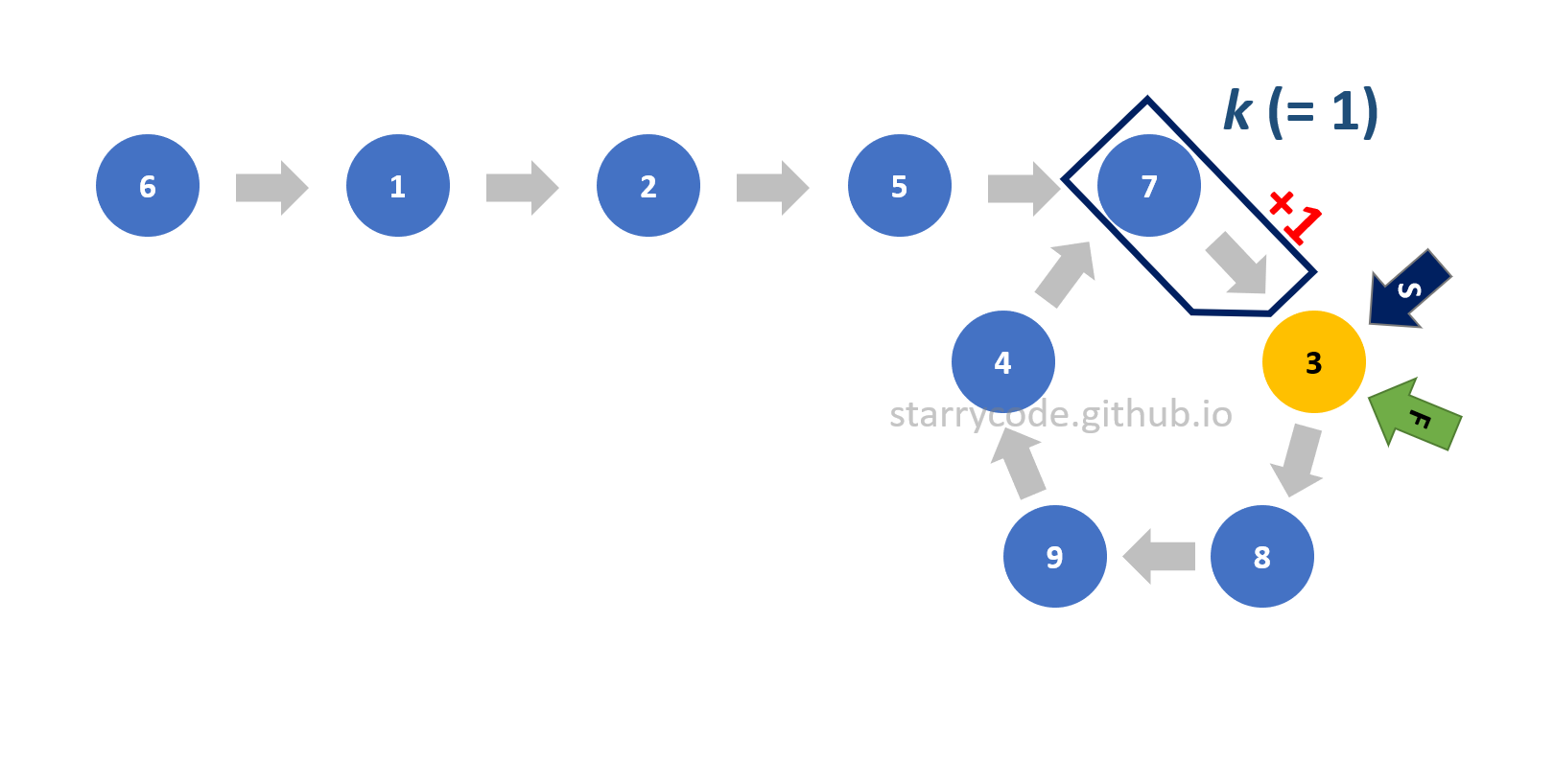
Figure 19: Algorithm explanation 2

Using these three variables, the distance traveled by the slower pointer is illustrated as the following:

Since the pointer traveled from the start of the list, entered the loop and looped p times, and k amount since that is the end of the travel.

Similarly, the distance traveled by the faster pointer is illustrated as the following:

Note that p is less than q since the speed of the faster pointer is faster than that of the slower pointer and therefore the faster pointer travels more than the slower pointer.

Since the faster pointer traveled twice as fast as the slower pointer, the distance traveled by the faster pointer is as twice as the distance traveled by the slower pointer as well.

By simplifying the above equation, it is equivalent to the following:

Which implies that m + k is a multiple of l. Note that (q - 2p) will be replaced with x.

Hence, by the time the slower pointer entered the loop and traveled the distance of m, the faster pointer had also traveled the distance of m, or x * l – k since both pointers are moving at the same pace. Since m + k is a multiple of l and the faster pointer started from k, both pointers meet at the start of the loop.

1.4. Code Implementation¶

            
               # Author: Violet Oh
                Class ListNode:
                    def __init__(self, x):
                        self.val = x
                        self.next = None
                Class LinkedList:
                    def hasCycle(self, head:ListNode) -> bool:
                        slow = fast = head
                        while fast and fast.next:
                            slow = slow.next
                            fast = fast.next.next
                            if fast == slow:               
                                return True
                        return False

                # Create a linked list
                linked_list = LinkedList()
                linked_list.push(4)
                linked_list.push(9)
                linked_list.push(8)
                linked_list.push(3)
                linked_list.push(7)
                linked_list.push(5)
                linked_list.push(2)
                linked_list.push(1)
                linked_list.push(6)
                answer = linked_list.hasCycle(linked_list.head)
                print(answer)

                # Make a loop inside the list
                linked_list.head.next.next.next.next.next.next.next.next.next = linked_list.head.next.next.next.next
                answer = linked_list.hasCycle(linked_list.head)
                print(answer)